|
Malhar Rajpal A few weeks ago, two extremely renowned mathematicians, Avi Wigderson and László Lovász, won the prestigious Abel Prize. Becoming an Abel Prize laureate is not an easy feat, since it is only awarded to the most accomplished mathematicians in a given year. Known colloquially as the Nobel Prize pf mathematics, it has a substantial cash prize of 7.5 million Norwegian Kroner. In this article, I will talk about one of the 2021 Abel Prize winners, László Lovász and his work.
On March 9, 1948, Lovász was born in Budapest, Hungary. He was an extremely talented mathematician from an early age and managed to win three gold medals and a silver medal at the renowned International Mathematical Olympiad, the most competitive and largest high school math competition in the world, where countries send teams of their six best mathematicians to compete. Winning a medal is not an easy feat with only around the top 8% of already brilliant participants receiving a gold medal. Achieving four medals, thus, is quite an amazing achievement and truly showed Lovász’s outstanding mathematical ability at a young age. As a prodigious mathematician, he had the opportunity to meet and learn about game theory from Paul Erdös in his youth. After studying mathematics at the undergraduate and postgraduate level at Hungary's top universities, Lovász became increasingly prominent as a researcher in the field of mathematics and computer science. He worked under the supervision of Tibor Gallai through his doctoral research in the 1970s. He also worked closely with Erdös to develop methods to complement Erdös’ graph theory techniques. One of his largest accomplishments was developing the Lovász local lemma in graph theory which states that as long as a certain number of events are ‘mostly’ independent from each other, and aren’t individually very likely, then there will be a probability that none of them occurs. Of course, there are several intricacies to this lemma that are beyond the scope of this article but it was a vital development because it led to breakthroughs in creating existential proofs for rare graphs and is used in the probabilistic method. Relating to graph theory, he also contributed to the formulation of the Erdös-Faber-Lovász conjecture in 1972 which stated that ‘If k complete graphs, each having exactly k vertices, have the property that every pair of complete graphs has at most one shared vertex, then the union of the graphs can be properly colored with k colors’. This conjecture remains unsolved, however, in 2021, a proof of the conjecture was made for all sufficiently large values of k by a team of five researchers. He also proved Kneser’s conjecture in 1978, where Martin Kneser conjectured in 1955 that the chromatic number (the minimum number of colours needed to colour the nodes of a graph such that no two nodes that share an edge have the same colour) of the Kneser graph K(n, k), for n >= 2k is exactly n-2k+2. Lovász proved it by using topological methods which was significant because it made developments to the huge field of topological combinatorics. Further, in 1982, Lovász worked with Arjen Lenstra and Hendrik Lenstra to create the LLL algorithm which is a polynomial time reduction algorithm. This algorithm was a huge breakthrough for Lovász since it led to massive developments in cryptography and polynomial factorisation, the basis of RSA cryptography. This is, by no means, an exhaustive list of Lovász’s numerous accomplishments, and Lovász has made a considerable impact in the fields of mathematics and computer science over the last five decades. He has been rewarded with several prestigious awards and has worked in numerous outstanding institutions including Yale University, Microsoft Research Center, and the Hungarian Academy of Sciences. His Abel Prize for significant contributions to theoretical computer science and discrete mathematics is therefore fully deserved.
0 Comments
Nitya Nigam Since the advent of modern computing in the 1950s, computers have played an essential role in mathematical research. They're often used to test conjectures, as they can iterate through long lists of numbers extremely quickly to check whether they satisfy the conditions that have been predicted. They are also used to find specific types of numbers, such as Mersenne primes (you can even join the Great Internet Mersenne Prime Search yourself). However, coming up with conjectures has long been the work of mathematicians themselves. A good mathematical conjecture states something profound and useful within the field. It must be interesting enough to prompt investigation, but not so niche as to have very narrow applications. Getting computers to strike this balance is therefore a tall task.
However, researchers at the Technion in Israel have created an automated conjecturing system called the Ramanujan Machine, named after the famous mathematician Srinivasa Ramanujan. The software has already conjectured original formulas for several mathematical constants (published in this Nature article) including Catalan's number and pi. The software works by leveraging the fact that many such constants are equal to continued fractions (fractions where the denominator is the sum of two terms, one of which is a fraction with a denominator that also contains a fraction, and so on until infinity). Continued fractions have been of mathematical interest both for their aesthetics and what they reveal about constants' fundamental properties. The software works by first finding continued fraction expressions that seem to equal universal constants by choosing arbitrary constants and expressions, then computing each side to a certain level of precision and seeing if they approach each other. If they seem to approach each other, they are computed to higher precision to ensure that it is not a coincidence. Since formulas already exist to compute pi and other constants to an arbitrary level of precision, the only thing in the way of making sure the sides match is computing time. So far, the software has conjectured a formula for Catalan's constant that allows for its fastest computation yet. This is an important milestone for computational mathematics, not just because it shows promise for developing faster methods to compute other constants, but because these automated conjectures may be used to reverse-engineer more theorems, further fueling mathematical innovation, Malhar Rajpal Last week's article outlined the underlying structures of depth first search. Check it out here before continuing with the rest of this article, which will describe how the algorithm actually works! By using the stack data structure, we must explore the last node that was added to the frontier. Since A in the table above is the only node in the frontier, it is also the last node that was added and is therefore explored. By the exploration process mentioned above, the algorithm first checks whether node A is the solution node. Since the program knows that node G is the solution, our algorithm deduces that node A is not the solution node. It, therefore, retrieves all the nodes connected to node A, namely node B and node C. It then checks if either of these nodes are in the explored nodes list. Since neither of them are, the program adds them to the frontier arbitrarily(let’s say C is added before B in this case, however it could also be the other way around). Node B and C also have a link to their parent element, node A stored inside of them. Node A is then removed from the frontier and added to the explored nodes list: 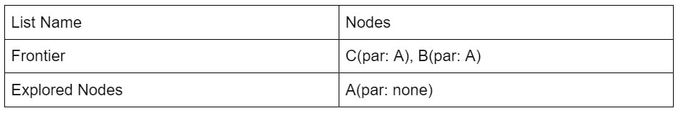 Since B was the last node to be added to the frontier, by the rules of the stack, it is the next node to be explored. By using the same process as above, we see that node B is not the solution node. The nodes directly connected to B, nodes A and E, are retrieved. Since node A is already in the explored nodes list, it is ignored. Node E, which isn’t in the frontier or the explored nodes list is then added to the frontier. Node B is then transferred to the explored nodes list: 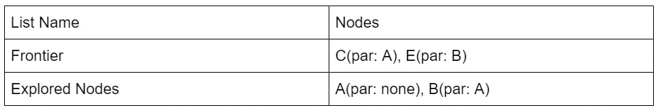 If you follow the same process as above, you should figure out that after exploring node E, no new nodes are added to the frontier(since node C is already in the frontier and node B is already explored). Thus we end up with the table: 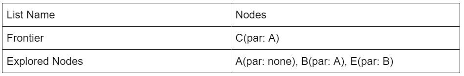 After exploring node C, two new nodes: node F and node D are added to the frontier(let’s assume in the order F then D). The other two nodes that connect with node C: node E and node A are ignored because they have already been explored. However, if you wish to code a more complex algorithm, you could show that since there is at least one explored node between node A and node C, since node C connects with node A, and since node C also directly connects with the previously explored node(E), there is a cycle in the graph. The length of this cycle could also be determined. 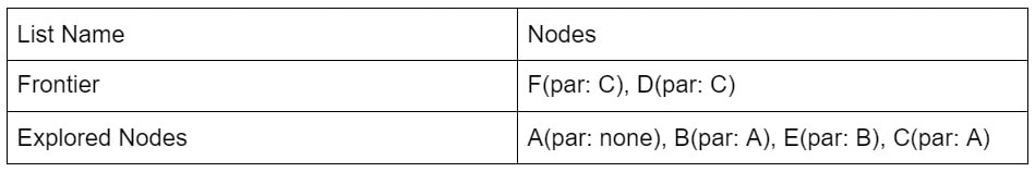 After exploring D, nothing new is added to the frontier. This is because the only node connecting node D is node C which had just been explored. Because of this, node D is classified as a ‘dead-end’. When a DFS algorithm reaches a dead-end, it backtracks to the last decision point and follow the path resulting from another choice:
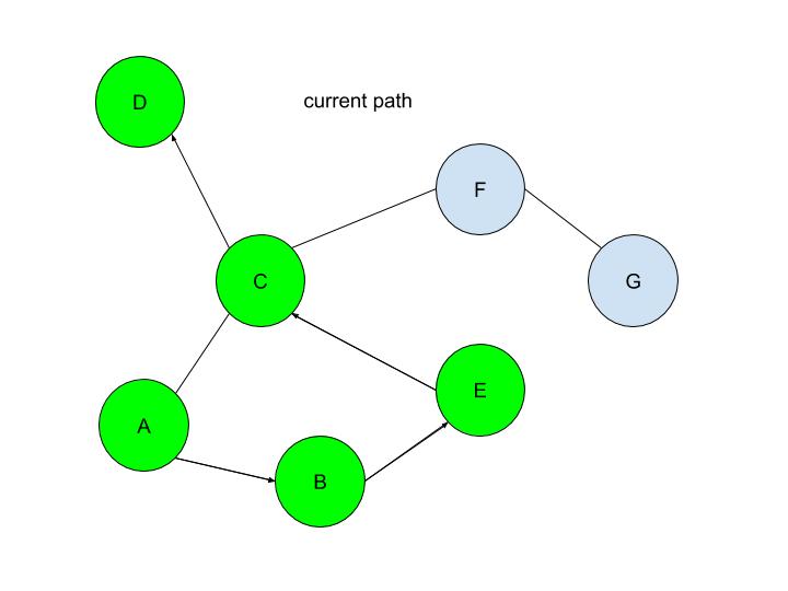
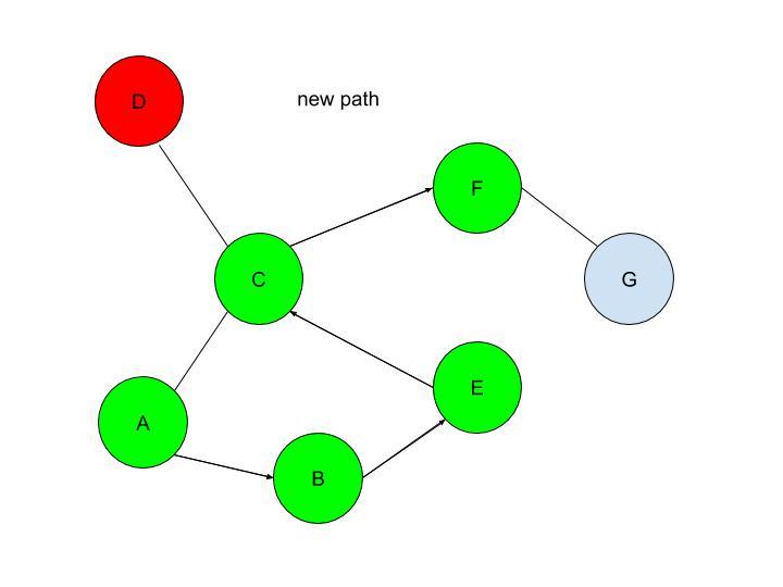
We see that after DFS sees that node D is a dead-end, it backtracks to the last decision point(node C), and makes the other decision(traversing to node F). This is automatically done through the stack frontier procedure described above. 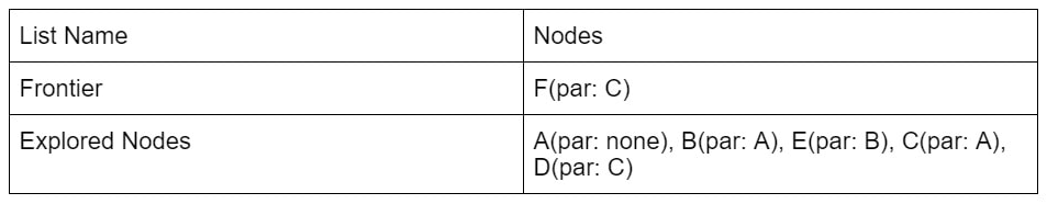 Node F is then explored and it is evident that node G is the only node that is added to the frontier: 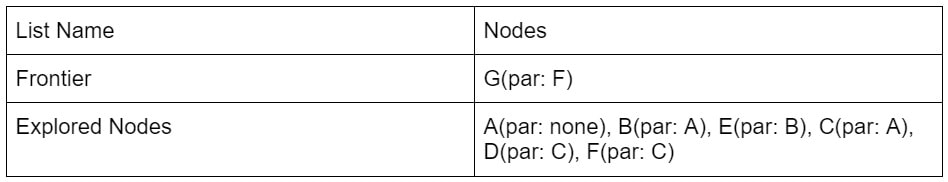 Now our exploration process checks Node G against the solution and it determines that Node G is in fact our goal node! Since we kept track of the parents, we can easily backtrack the optimal route from the solution node(Node G) all the way to the initial Node. We can do this by creating a list and adding the subsequent parent elements of each of the previous nodes to the list, until we reach node A(which has par:none). Hence from Node G, we go to it’s parent, Node F, then to its parent, Node C, and continue until we reach Node A. This gives us this list: (G, F, C, A). Reversing this list, we can find a route to node G: (Node A → Node C → Node F → Node G)!
If the problem was more complex, stacks would have ensured that each branch was explored until a dead end was reached(such as node D in this case), before backtracking to the last possible decision point(a node connecting to several other nodes) and exploring another branch from there(by traversing to a different node than it did initially). DFS is a powerful, uninformed search algorithm that can be used in a variety of situations, such as solving single solutioned maze problems, performing topological sorting, and is even used in Minimax, which is shown in one of my previous articles! It also sets the foundation of better, more efficient heuristic functions (such as greedy best first search or A* search which are informed search algorithms). If you have read my article on BFS, you may be wondering, when you should use BFS over DFS, or vice versa. Don’t fret, because in my next article, I will evaluate the strengths and weaknesses of both the algorithms! Malhar Rajpal This is the first of a two-article piece on depth first search. From performing topological sorting to solving puzzles with one solution(such as mazes), depth first search is a powerful search algorithm that can be used to crack a large variety of problems. In any puzzle, for example a maze, depth-first search (DFS) works by exploring one route in its entirety (until a dead-end is reached or the solution is obtained). If the solution is obtained, it returns the correct path. If not, the algorithm is programmed to backtrack and try out another route in its entirety, performing the same process. To perform this, DFS uses a data structure called a stack, which is a last in, first out data type (don’t worry if you don’t understand this yet). The puzzle: To explain the concept of a stack and DFS, I will use an unweighted graph: 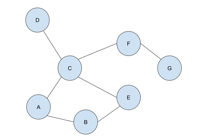 Let’s assume we start at circle A on the unweighted graph and we want to make our way to circle G. We can visualise this as a simple maze, where every line (or edge more formally) that connects two circles (more formally called nodes) is a possible move from one place to the next. Nodes with no edges connecting it except for the one that led to it (such as node D) can be considered as a ‘dead end’. Our goal is to use the DFS algorithm to find the route from starting point, node A, to the end of the maze, node G. Obviously, since this maze is very simple, we can visually see that the answer is A → C → F → G, however we want to know how an algorithm can figure this out, and how this method can be used to solve more complex puzzles that we perhaps couldn’t solve visually. Initialising the algorithm: The DFS algorithm requires a list which is more formally called the frontier. This frontier contains the nodes that are currently being explored or will be explored in the future (unless the solution is reached before the node can be explored). Another list containing the already explored nodes is also needed. When we begin running the algorithm, our initial node A is put into the frontier (shown below), since it is the first node that will be explored. Since no nodes have been explored yet, the list containing the explored nodes remains empty.  Stacks:
The stack data structure used for DFS is a last in, first out data type. Simply put, this means that the frontier will explore and remove the node that was last appended to the frontier list. This explored node then gets transferred to the explored nodes list. But what exactly do we mean by ‘the frontier will explore’ a node? The exploration process: Exploring a node includes checking if the currently explored node is equal to the solution node (in this case node G) or if node ‘solution node’ is explicitly stated, then by checking whether the currently explored node follows all the conditions in a predetermined set of criteria that defines the solution (criteria such as the solution node must be connected to node F and no other node). If it is deduced that the current node is the solution node, then the program can return the path needed to reach the final node. If it is not, then all the nodes that connect with the current node are retrieved. A check is performed on each of the connected nodes: if the node has already been explored (if it’s in the explored nodes list already) and if it’s not already in the frontier, then it is ignored. If it hasn’t been explored, then it will be added to the frontier. The order of the connected nodes being added to the frontier is completely arbitrary in DFS. The node has now been explored and is thus moved from the frontier list to the explored nodes list. The nodes: Each node stores its needed data (whatever it may be) as well as the parent node within itself. For example, Node B contains its own information as well as that of its parent element (Node A). These parents will be labelled in our table using the format ‘par: letter of node’ (appearing in my next article). This is to back-track and find the correct path from the initial position to the solution once the solution node is reached. The parent node of some node is easily found: we can refer to the parent node of some node as the node which was being explored right when this new node was first brought to the frontier. Check out my next article to see how the algorithm works on an example! Nitya Nigam A few weeks ago, we wrote about end-to-end encryption and examined the maths behind the Diffie-Hellman key exchange. Continuing on the theme of cryptography, today’s article will talk about pseudorandomness, an important concept to many fields, including complexity theory, combinatorics, number theory, and, of course, cryptography. This article hopes to leave you with a fundamental understanding of why pseudorandomness is so important, and the structures that underpin its study.
Firstly, what is pseudorandomness? As you can probably guess from its word root, it essentially means “fake randomness”. True randomness, as is seen in radioactive decay and quantum phenomena, cannot be truly replicated by computers, which are deterministic - they run on Boolean logic (let us know in the comments if you’d like to read an article about this), not probability. But being able to replicate randomness is an important tool for mathematicians and computer scientists alike. It has applications as simple as generating winning lottery numbers and as complex as simulating nuclear fission. In these situations and more, it is important to have a way to generate numbers in an unpredictable pattern. As we discussed in our article on encryption, messages can be made secret using keys. Cryptosystems are most secure when these keys are random, so that they cannot easily be guessed by an interceptor, which is why randomness is so important in the field. Pseudorandom number generators rely on a special type of mathematical concept called one-way functions. These are functions that are easy to perform in one direction, but are near-impossible to reverse. The process of modular exponentiation discussed in our encryption article is an example of a one-way function, but the most commonly cited example of such functions is multiplying two large prime numbers together. This is an easy process, but factoring the large product back into its prime components is very computationally inefficient. There are three steps that link pseudorandom number generators to one-way functions. First, let’s define our generator, G, as unpredictable if every polynomial-time algorithm struggles to predict the nth number from the first n-1 numbers. Note that this definition only covers numbers already generated, and doesn’t extend to how generators actually generate new numbers. That is where one-way functions come in. For G to be pseudorandom, it must first be unpredictable. However, if G is not pseudorandom, then G is predictable. If G is not pseudorandom, then there must be some algorithm that can distinguish between outputs of G and a uniformly sampled string with non-negligible accuracy, and a bit of maths too complicated for us to cover called Yao’s Theorem states that the latter cannot be the case, so all unpredictable generators are also pseudorandom. To turn G into a proper generator, we need to show that it is possible for G to generate new numbers that cannot be predicted to a non-negligible degree of accuracy. The Goldreich-Levin Theorem (the proof of which is also too complex to go into here) states that one-way functions can be used to stretch the output of a generator by one number, allowing for pseudorandomness to be achieved. Our generator G needs a number called a pseudorandom seed to get started, as one-way functions can only extend strings, not create them. If this seed is kept secret, though, such generators serve as effective ways of generating random keys for encrypted communication. Understanding pseudorandomness also has more tangible benefits. In 2003, Mohan Srivastava, a statistician in Canada, discovered that the Ontario Lottery was using a pseudorandom number generator for its scratch cards, so cards with a row containing three numbers that each appear only once within the card’s visible numbers were almost always winners. This is because pseudorandomness follows a specific probability distribution, based on the one-way function it uses. Instead of gaming the system and keeping the money for himself, Srivastava sent the Ontario Lottery and Gaming Corporation 20 unscratched cards, each marked as either winners or losers. Two hours later, he got a call telling him he had correctly identified 19 out of the 20 cards. The game was discontinued the next day. I hope this article has left you with a better understanding of pseudorandomness and its uses. Let us know in the comments if you have any questions, and tell us what you’d like to read about next! Malhar Rajpal Imagine you have a complex maze with hundreds of ways to reach the endpoint. How do you find the shortest route? This is the exact problem that appears in a vast array of real-world problems from GPS navigation to tracing garbage collection. You could split the problem into an unweighted graph, where each position in the maze or street on the map is a node, and try to manually trace the different solutions from the initial position (also known as the root node) to the solution. But you will soon find that, since there are so many different routes, solving this problem manually is a near-impossible task! You need to use a computer algorithm, and luckily for you, the solution comes in the form of Breadth First Search (BFS), which explores each node in the unweighted graph until the solution is reached. To explain the concept of BFS, I will use a basic example: 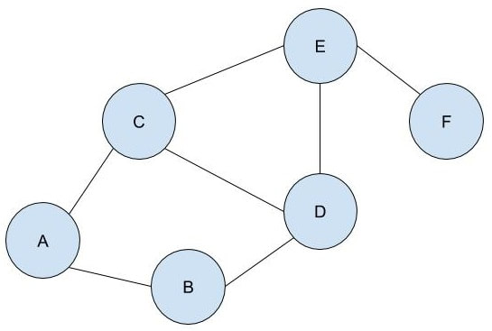 L circle (node) A be our root node, and we must traverse our way to node F, which is our end node, or solution. We could analogise each of the nodes in the graph to be a certain street, and each of the lines show which streets are connected (for example street A is directly connected to street B or street C). There are obviously several ways to get from node A to node F (two of which could be A → B → D → E → F or A → C → D → E → F), but we want to get to node F by traversing through the least amount of nodes or streets. How would the algorithm do this? The answer is not as complex as you may think. The algorithm requires a list (more formally called a frontier). This frontier contains the nodes that are currently being explored. Another list is also needed which contains the explored nodes. When the algorithm initialises, node A (our first node) is put into our frontier (as shown below) since it is the first to be explored. The list containing the explored nodes remains empty. 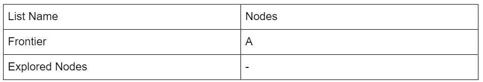 The frontier makes use of a queue data structure which, simply put, will always explore the first node that was appended in a list (in this case our frontier). Since node A is our only node, and hence the first node, it is explored. The exploration process includes checking if the current node is equal to the solution node. If it is, then the program can return the path needed to reach the final node. If not, the program will check if any of the directly connected nodes to the current node is in the ‘Explored Nodes’ list. The program will then simply add all the connected nodes that are not in the ‘Explored Nodes’ list to the frontier. So in our example, since node B and C are directed connected to A, and since neither node B or C are in the explored nodes list, they are both added to the frontier like so: Since node A is now explored and a queue is a first in first out data structure, meaning the first node in the list is the node that is removed when needed (when a node is removed from a queue, it can only be the first first node in the list). Node A is then added to the explored nodes: Each node contains the needed data (street name etc.) as well as the parent node within itself. For example, node B contains its own information as well as its parent element (node A). These parents will be labelled in our table using the format ‘par: letter of node’. Now, since node B is the first node in our frontier, it follows the same process as before: it is checked whether it is the solution node (node F). Since it’s not, the program gets all its connected nodes: node A and node D. Since node A is already explored, it is ignored (this avoids backtracking) and node D (with its parent being node B) is added to the frontier. Node B is then added to the explored nodes. This process is continued until we arrive at the following table: Finally node F is our solution. Since we kept track of the parents, we can easily backtrack the optimal route from the solution node (Node F) all the way to the initial node. We can do this by creating a list and adding the subsequent parent elements of each of the previous nodes to the list, until we reach node A (which has par:none). This gives us this list: (F, E, C, A). Reversing this list, we can find the shortest route to node F: Node A → Node C → Node E → Node F (shown in red on the below diagram), which only traverses through four nodes! This is great since our programs can easily perform each exploration in a matter of milliseconds, allowing incredibly complex search problems to be entirely solved in as little as a couple of seconds! 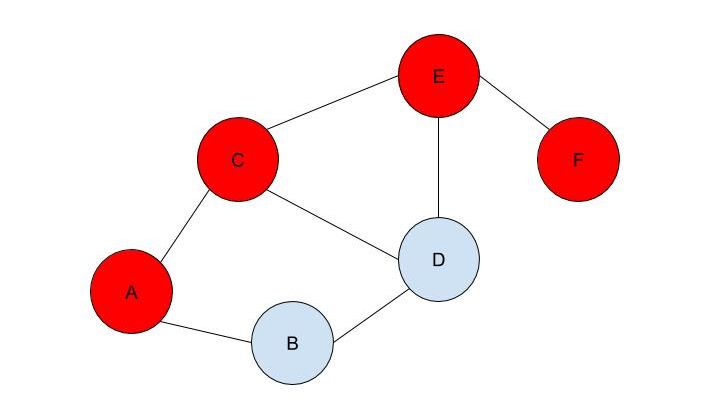 BFS is a widely used algorithm, effective in finding the shortest route from one node to another. Although complex problems like GPS navigation systems use slightly different algorithms since they must take into account several different aspects (traffic, speed limits etc.), these algorithms are all built upon the fundamental principles of BFS. If you want to go deeper into the world of search algorithms, I would suggest looking at A* search, which finds the route between two nodes with the lowest cost (cost referring to some variable; it could be lowest time, lowest distance etc.).
Nitya Nigam Internet privacy is an important and relevant issue in today’s world, especially given recent moves by world governments to restrict the influence of foreign technology companies in their countries. This is why Integral has partnered with Bytesized Privacy to give our readers insight into encryption, one of the most effective ways to ensure private data stays private. This article will cover the maths behind the Diffie-Hellman key exchange, which is a secure and widely used method of public key cryptography. Bytesized has a post about the applications as well as the pros and cons of end-to-end encryption that you can find here. We hope you find this collaboration useful and interesting. Let us know in the comments if you’d like to see more posts like this!
Public key cryptography is a type of encryption where each person has a pair of cryptographic keys: a public key and a private key. The private key is kept secret, but the public key can be used by anybody. The Diffie-Hellman key exchange uses public and private keys to give both sender and receiver a shared key that can be used in future communications, as the process of using both public and private keys for every message is computationally expensive. The maths behind this key exchange is based in modular arithmetic, where integers that have the same remainder when divided by a set integer are considered the same, or “congruent”. We can notate this mathematically by saying that, for example, 6 ≡ 1 mod 5, where the ≡ symbol means “congruent to”, mod means modulo (x mod y means x is the remainder when a number is divided by y) and 5 is the set integer we are using as the base of this system. The Diffie-Hellman key exchange involves 5 steps, outlined below. Let our two people who want to communicate with each other be called Alice and Bob.
Alice and Bob now have a shared key, s, that they can use for secure communication, that is unknown to all other users. This method works because B ≡ g^b mod p and A ≡ g^a mod p, so B^a ≡ g^ba mod p and A^b ≡ g^ab mod p, which are equivalent. This method is secure because for large p, a and b, reversing the modular exponentiation is near-impossible via a brute force attack, because there are many different possible values of base and exponent that lead to the same value after reducing the result mod p. g is usually quite small, as most primitive roots are small integers like 2 and 3. g being small does not compromise the security of the system. Malhar Rajpal As seen in my previous article (reading it will help you understand this article), Minimax is a fantastic way to program game engines so that they play effectively. However, for more complex games, like chess, Minimax would take far too long to find the optimal move, even if it’s only looking 4 or 5 moves ahead! This speed problem, however, can be easily resolved with alpha-beta pruning. Alpha-beta pruning is a search algorithm that explores less nodes (triangles) than Minimax does while still outputting the same best action for the player. It does this by evaluating the score of one node from a group of previous nodes at a time (similar to Minimax). However, upon evaluating the score of another node, if the output score is proven to be worse than other previously explored output scores before some of its child nodes are even considered, then the program doesn’t bother exploring these child nodes, therefore saving time. In other words, it returns the same move as Minimax while removing (or pruning) irrelevant nodes before they are examined. This sounds very complex but I assure you that after you read the example, you will find that it is actually a very simple concept! Let’s take a look at a Minimax diagram similar to the one shown in my Minimax article in which each player has three possible choices. I have given arbitrary values for each of the 9 possible outcomes resulting 2 actions ahead from the initial move (or root node). 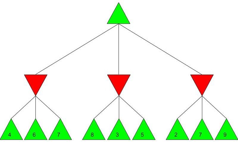 For the first minimizing node (triangle) from the left, we can do it the same way as we did using Minimax. Since the minimizing player will always choose the lowest possible option (since it is playing optimally), out of the possible scores of 4, 6, 7, the minimizing player will choose 4, as shown in the diagram below: This is the exact same as Minimax! But for the middle minimizing node, the algorithm first explores the child node with a score of 8, then the node with a score of 3. Since 3 is less than 8, and it’s the minimizing player’s turn, the algorithm will prefer the node with the score of 3. We can also, however, see that 3 is less than the 4 from the leftmost minimizing node. This means that even without considering the node with value of 5, we can say that the middle minimizing node must have a score that is less than or equal to 3(<=3), since the minimizing player will always choose the lowest possible score. We don’t need to consider the node with value of 5 because the node with a score of 4 from the left is greater than the already explored node with score 3, hence for the root node, the maximising player will prefer the node with score 4 over the score of the middle node which can be said to be <= 3. In other words, there is no possible score for the node coloured blue below, that would change the decision of the root node. 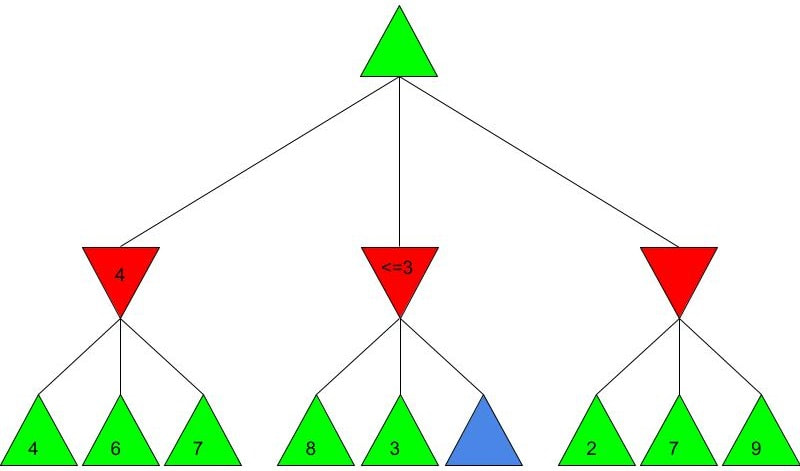 We, therefore, can prune the node coloured blue and any potential nodes that branch below it, hence saving a lot of time! I put <=3 in the middle minimizing triangle for clarity, however the program will not need to consider it when evaluating the score for the root node since the maximising player always prefers the node with a score of 4 over the <=3 score in the middle minimizing triangle, so we can just eliminate this branch entirely. Now we can calculate the rightmost minimizing triangle. Immediately we see a node with the score of 2. So we can immediately say that the rightmost minimizing node must have a score of <=2 (since the minimizing player will always choose the lowest score). Since the next move, made by the maximising player, will always prefer the score of 4 in the leftmost minimizing node over the <=2, we don’t even need to consider looking at the nodes with scores of 7 and 9. Eliminating these nodes and the nodes that could branch off below them without even exploring them saves even more time! 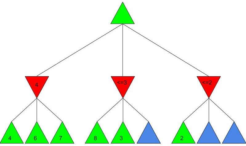 When we prune a node, that means that we don’t need to consider its parent node either. We can therefore eliminate that entire branch too, since if a child node is pruned, its parent node will not be preferred as compared to one of its aunt/uncle nodes. So when we prune the sixth, eight and ninth nodes from the left, we can subsequently eliminate its parent node too: 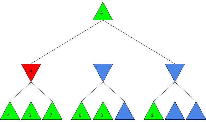 Now since the root node only needs to consider the node with value 4, it will be chosen (as shown above) without even considering the other nodes, further cutting down on algorithm runtime. If you were to try and evaluate the Minimax tree as we did in the previous article, you would find that the score in the root node would be the same. The only difference would be that, when programmed, the alpha-beta pruning algorithm would take substantially less time.
Alpha-beta pruning is a powerful algorithm that can be used to program game engines in an even more efficient manner. When used with depth-limited Minimax, alpha-beta pruning can be used to make engines quickly play near-optimal moves in games as complex as chess! Malhar Rajpal What do games like chess, Go and tic-tac-toe have in common? They are all based on choices. On a daily basis, humans train their decision making skills numerous times, making selections that can be as simple as figuring out when to go to bed or as complex as evaluating the quickest route from one place to another. Despite our evident practice in decision-making, artificial intelligence still crushes humans in games such as chess. Since computers are programmed by humans, you may wonder how it is possible that they can make much better choices in complex games that are nigh-impossible for any human to master. The answer is minimax. Minimax is a decision making rule that is widely used to program AI to make better actions/choices. Its foundation is based on creating an overall score of the game so the AI can see who’s ‘winning’ at any given position. Although most games don’t have an explicit score while the game is in progress (only a winner and loser at the end), coming up with a score system is not difficult. Score systems can be quite simple: for example in chess, we can give each piece a certain score (e.g. rook/knight = 5 points and queen = 9 points) and then sum up the scores of the pieces on the board for both players at a given point in time, and then subtract the score for player 2 from the score for player 1 (player 1 - player 2). If the final value is positive, then player 1 is winning, but if it is negative, then player 2 is winning. If the score is 0 then the position is equal. The higher the score, the larger the margin by which player 1 is winning. Likewise, the lower the score, the larger the margin by which player 2 is winning. Now that we understand how scoring works, we can move onto the algorithm. Imagine programming an engine to play a simple two player game, where each player has only three decisions. As seen before, player 1 wants the evaluated score to be positive, and as high as possible. Player 1 is therefore called the ‘maximising player’ or ‘max player’. On the contrary, player 2 wants a negative score that is as low as possible, so they are the ‘minimising player’ or ‘min player’. Now let’s look at the Minimax tree diagram shown below this paragraph. Every triangle in the diagram represents a certain state or position and is formally called a ‘node’. Each green, upwards triangle indicates a maximising state/position - that is, given some potential scores in the branches below it, the ‘max’ player will always choose the highest one. Each red, downward triangle indicates a minimizing state/position - given some potential scores in the branches below it, the ‘min’ player will always choose the lowest one. These chosen scores will then be assigned to their respective triangles in the diagram. Finally, each branch, or line, connecting two triangles represents a potential move/action. 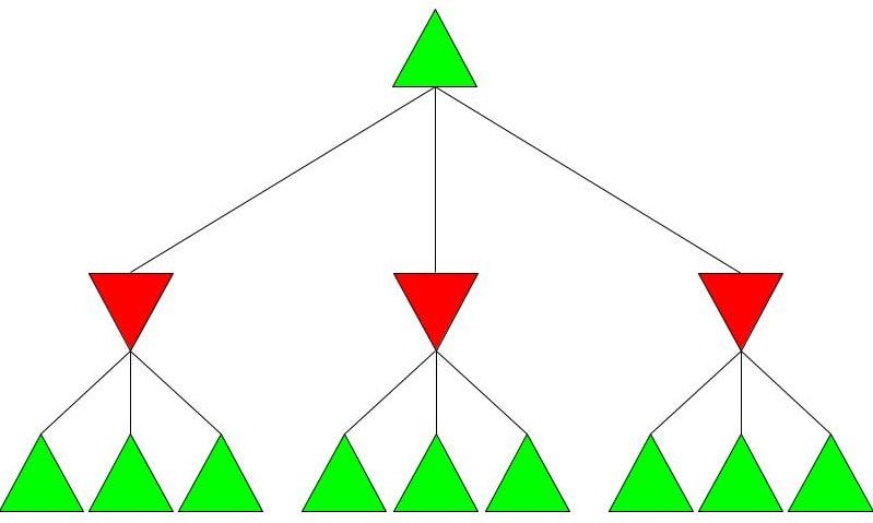 Since the top triangle (formally called the ‘root node’) represents a maximising state, the goal in the diagram is to find the best move for the max player. To do that, we have to find the highest possible score for the root node (assuming optimal play) and play the move that gives us this score. Each player has three decisions at every turn, so we can see that from the top, maximising triangle, we have three minimising triangles that branch off it. Likewise, for each minimising triangle, we have three more maximising triangles branching off it. Now, shown by the diagram below, our minimax program would ‘look’ into every possible position that is two moves ahead and calculate a score for each of the 9 possible positions. Since we are not playing a real game, I have assigned some arbitrary scores for each of the 9 positions: 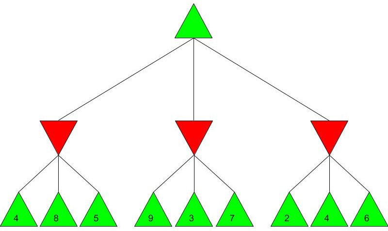 For each of the red minimising triangles or states, we have three scores assigned below them. For the leftmost minimising state, the min player has three choices: one choice gives the min player a score of 4, another gives a score of 8 and the final choice gives a score of 5. Since the minimising player wants to choose the minimum score and we must always assume that both players play optimally (the max player will always choose the highest choice and the min player will always choose the lowest choice in a minimax tree), the red triangles are therefore filled up as shown in the diagram below the paragraph. For the first minimising state, out of the possible positions evaluated as 4, 8, and 5, the minimising player, when playing optimally, will always choose the move that evaluates as the lowest score, hence choosing the move that results in score 4. This principle is the same for the other two triangles shown for the minimising player. 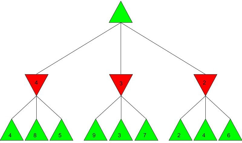 Finally, from the three minimising positions with the scores 4, 3, and 2, the maximising player will always choose the highest possible choice. The max player, which represents our program, therefore chooses the position which gives a score of 4, and plays the move which is assigned to it, labelled below: 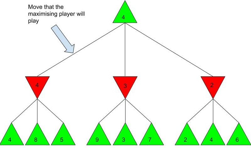 The example shown above is an example of depth-limited minimax. The depth for the minimax shown above is 2 since we evaluated all the possible positions 2 moves ahead, followed by an evaluation of all the possible positions 1 move ahead which was then used to figure out the move that the program plays. This is a repetitive process where the score for the positions less than x moves away are used to evaluate the score for the position x-1 positions away, until we reach the current position and therefore evaluate the best move. Because of this property, the minimax function is a recursive function. It is also an example of a depth first search algorithm.
Depth-limited minimax is used when the game has too many possibilities for the computer to evaluate every single position from start to end. This kind of function is used in games like chess which have over 13^64 possible positions. Depth-limited minimax, although faster, doesn’t always play the optimal move in certain positions. The higher the depth, the higher the chance of the computer playing an optimal move. Minimax without depth, however, will always play the best move. Minimax without depth is used in games like tic-tac-toe where there aren’t that many possible positions. Minimax without depth works similarly, except that the AI is programmed to evaluate every single position from start until the end and find a forced win that happens in the least number of moves possible. Minimax is widely used to create game engines. However, you may realise that for complex games like chess, depth limits above 3 can take a huge amount of time with just minimax. To counter that, programmers use a process called alpha-beta pruning which drastically reduces the amount of time needed. Alpha-beta pruning, used along with minimax, can be used to create game engines that are much smarter than any human is. Sayonee Das As far back as the time of the ancient Greeks, mathematicians have studied whole numbers and their properties. This branch of maths is called number theory, and is one of the oldest mathematical fields. To this day, there are open questions in number theory, which demonstrates its complexity.
One source of such open questions is the study of perfect numbers. A perfect number is a whole number (integer) which equals the sum of its proper divisors. For example, 6 is divisible by 1, 2, and 3 and it’s also equal to their sum as 1 + 2 + 3 = 6. Likewise, 28 is divisible by 1, 2, 4, 7, and 14 and it’s equal to 1 + 2 + 4 + 7 + 14 = 28. The simplicity of what defines perfect numbers makes them easily understandable to non-mathematicians, so their study intrigues mathematicians and non-mathematicians alike. Perfect numbers were first studied around 300BC when Euclid first proved that if (2^p − 1) is prime then (2^(p−1))(2^p − 1) is perfect. The first four perfect numbers were the only ones known to early Greek mathematicians. Throughout history, many more mathematicians played a role in bettering our understanding of perfect numbers. One of them was Ibn al-Haytham, who first suggested that the opposite (converse) of Euclid's theorem was also true: not only do numbers of the form (2^p − 1) generate perfect numbers, but all even perfect numbers are generated this way. This was eventually proven by Euler in the 1700s. A clear, animated explanation of this proof is linked here. Today, 51 perfect numbers have been discovered, with the largest having 49,724,095 digits - over three million more digits than the 50th perfect number! Even though new even perfect numbers are discovered almost every year, some questions still remain:
Infinite even perfect numbers Sometimes we see prime numbers that have the form (2^p − 1), where p is a prime number. These numbers are called Mersenne primes. As mentioned above, Euclid proved that if (2^p − 1) is a Mersenne prime, then (2^(p−1))(2^p − 1) is a perfect number. From this, we can see that the questions of the infinitude of Mersenne primes that of perfect numbers are linked. By proving the existence of infinite Mersenne primes, we can prove the existence of infinite even perfect numbers. Currently, no proof in either direction - that there are either a finite or an infinite number of Mersenne primes - exists. Mathematical consensus, based on empirical data and heuristic methods using harmonic series, is generally that there are likely to be an infinite number of Mersenne primes, and therefore even perfect numbers, but a concrete proof of this remains to be found. Odd perfect numbers Whether or not odd perfect numbers exist hasn’t been proven either. However, people have proved properties that odd perfect numbers must have, if there are any. Although the requirements for odd perfect numbers have become more demanding, they’re not contradictory and so it remains logically possible that such numbers exist. Yet, most experts believe that odd perfect numbers don’t exist. Wikipedia lists the properties that odd numbers must have; if you were to look at them, their rigidity would surprise you - I know I was! Among the many others, one property listed is that an odd perfect number must have at least 300 digits. Computers have been testing odd numbers to see it they are perfect for decades now, but have yet to find any odd perfect numbers. Although computer testing would be a valid way to disprove the conjecture that no odd perfect numbers exist, as a counterexample would disprove the claim, if there are indeed no perfect numbers, computer testing will not provide us with any real knowledge. Even if we test a vast number of odd numbers, we will not be able to conclusively state that the next odd number isn't perfect, so a concrete mathematical proof is required. Let us know in the comments if you enjoyed this discussion of perfect numbers, and what you'd like to see us talk about next! |