|
Malhar Rajpal This is the first of a two-article piece on depth first search. From performing topological sorting to solving puzzles with one solution(such as mazes), depth first search is a powerful search algorithm that can be used to crack a large variety of problems. In any puzzle, for example a maze, depth-first search (DFS) works by exploring one route in its entirety (until a dead-end is reached or the solution is obtained). If the solution is obtained, it returns the correct path. If not, the algorithm is programmed to backtrack and try out another route in its entirety, performing the same process. To perform this, DFS uses a data structure called a stack, which is a last in, first out data type (don’t worry if you don’t understand this yet). The puzzle: To explain the concept of a stack and DFS, I will use an unweighted graph: 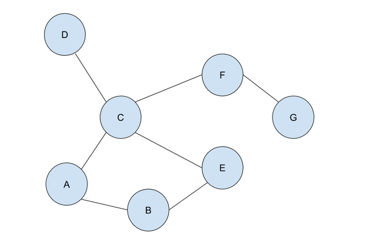 Let’s assume we start at circle A on the unweighted graph and we want to make our way to circle G. We can visualise this as a simple maze, where every line (or edge more formally) that connects two circles (more formally called nodes) is a possible move from one place to the next. Nodes with no edges connecting it except for the one that led to it (such as node D) can be considered as a ‘dead end’. Our goal is to use the DFS algorithm to find the route from starting point, node A, to the end of the maze, node G. Obviously, since this maze is very simple, we can visually see that the answer is A → C → F → G, however we want to know how an algorithm can figure this out, and how this method can be used to solve more complex puzzles that we perhaps couldn’t solve visually. Initialising the algorithm: The DFS algorithm requires a list which is more formally called the frontier. This frontier contains the nodes that are currently being explored or will be explored in the future (unless the solution is reached before the node can be explored). Another list containing the already explored nodes is also needed. When we begin running the algorithm, our initial node A is put into the frontier (shown below), since it is the first node that will be explored. Since no nodes have been explored yet, the list containing the explored nodes remains empty.  Stacks:
The stack data structure used for DFS is a last in, first out data type. Simply put, this means that the frontier will explore and remove the node that was last appended to the frontier list. This explored node then gets transferred to the explored nodes list. But what exactly do we mean by ‘the frontier will explore’ a node? The exploration process: Exploring a node includes checking if the currently explored node is equal to the solution node (in this case node G) or if node ‘solution node’ is explicitly stated, then by checking whether the currently explored node follows all the conditions in a predetermined set of criteria that defines the solution (criteria such as the solution node must be connected to node F and no other node). If it is deduced that the current node is the solution node, then the program can return the path needed to reach the final node. If it is not, then all the nodes that connect with the current node are retrieved. A check is performed on each of the connected nodes: if the node has already been explored (if it’s in the explored nodes list already) and if it’s not already in the frontier, then it is ignored. If it hasn’t been explored, then it will be added to the frontier. The order of the connected nodes being added to the frontier is completely arbitrary in DFS. The node has now been explored and is thus moved from the frontier list to the explored nodes list. The nodes: Each node stores its needed data (whatever it may be) as well as the parent node within itself. For example, Node B contains its own information as well as that of its parent element (Node A). These parents will be labelled in our table using the format ‘par: letter of node’ (appearing in my next article). This is to back-track and find the correct path from the initial position to the solution once the solution node is reached. The parent node of some node is easily found: we can refer to the parent node of some node as the node which was being explored right when this new node was first brought to the frontier. Check out my next article to see how the algorithm works on an example!
0 Comments
Leave a Reply. |