|
Malhar Rajpal In my previous mental maths article I outlined a technique to quickly square two-digit numbers in your head, which is an invaluable skill in maths competitions. Today, we will look at a trick to quickly solve a familiar type of question: finding the day of the week for any given date in the 21st century. This article will describe the method while my next article will explain why it works. The method itself is quite straightforward. It follows the formula: Day of week code = Remainder of [(Date + Month Code + (Last two digits of year + 6) + Quotient of [Last two digits of year / 4]) / 7] This may look confusing at first but let’s break it down: Date: The number for date is simple, it’s simply the day of the month. For example during April 27th, the date would be 27 and during December 9th, the date would be 9. Month Code: The month code is a single digit number that is associated with every month of the year. I have listed the codes below in a table and the reasoning behind each of these codes will be explained in the next article. This will require a little bit of memorisation and I recommend using some kind of key word or phrase to help you remember each month's code, it’s not that difficult with some effort! 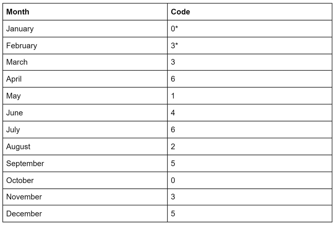 *On a leap year, the month codes for January and February become 6 and 2 respectively(1 less than their usual code) Remember that leap years occur on every year that is divisible by 4 except end of century years that are not divisible by 400. So 1904 and 2000 are leap years, yet 1900 is not because although it is divisible by 4, is an end of century year and isn’t divisible by 400. (Last two digits of year + 6) + Quotient of [Last two digits of year / 4]: The last two digits of year section is pretty self explanatory: for example if the year is 2024, the last two digits are 24, or if the year is 2001, the last two digits are 01. Make sure you add the +6 to the last two digits of the year - that is necessary to make the calculation correct. The quotient of [last two digits of year / 4] is simply the answer to the division problem of the last two digits / 4 without the remainder. So if the year is 2027, The quotient of [last two digits of year / 4] is the integer part of 27/4 = [6.75] = 6, and if the year is 2085, the quotient of [85 / 4] is 21. Putting it all together: Let’s take a random date in the 21st century, 6th May 2045, and try to find the day of the week. Using the formula: Day of week = Remainder of [(Date + Month Code + (Last two digits of year + 6) + Quotient of [Last two digits of year / 4]) / 7], We quickly see the date of May 6th 2045 is simply 6, the month code for May (referring to the table above) is 1, the last two digits of the year + 6 is simply 45 + 6 = 51, and the quotient of [last two digits of year/4] is [45/4] = 11. Plugging all of these numbers into the formula: Day of week code = Remainder of [(6 + 1 + 51 + 11)/7] = Remainder of [(69/7)]. The remainder of 69/7 is 6 since 69/7 is 9 with 6 leftover. And thus we get day of week = 6. What does this mean? To find out the day of the week, we follow this table: 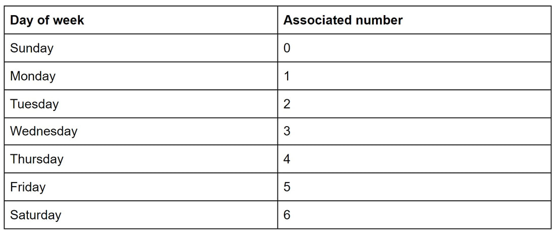 Since we got 6 as a remainder, we can use our table to figure out that the associated day of the week is Saturday. Hence, we can confidently say that May 6th, 2045 will occur on a Saturday!
Try it for yourself, choose a random date in the 21st century and try out the method! In the next article, I will prove why this formula works.
0 Comments
Malhar Rajpal A few weeks ago, two extremely renowned mathematicians, Avi Wigderson and László Lovász, won the prestigious Abel Prize. Becoming an Abel Prize laureate is not an easy feat, since it is only awarded to the most accomplished mathematicians in a given year. Known colloquially as the Nobel Prize pf mathematics, it has a substantial cash prize of 7.5 million Norwegian Kroner. In this article, I will talk about one of the 2021 Abel Prize winners, László Lovász and his work.
On March 9, 1948, Lovász was born in Budapest, Hungary. He was an extremely talented mathematician from an early age and managed to win three gold medals and a silver medal at the renowned International Mathematical Olympiad, the most competitive and largest high school math competition in the world, where countries send teams of their six best mathematicians to compete. Winning a medal is not an easy feat with only around the top 8% of already brilliant participants receiving a gold medal. Achieving four medals, thus, is quite an amazing achievement and truly showed Lovász’s outstanding mathematical ability at a young age. As a prodigious mathematician, he had the opportunity to meet and learn about game theory from Paul Erdös in his youth. After studying mathematics at the undergraduate and postgraduate level at Hungary's top universities, Lovász became increasingly prominent as a researcher in the field of mathematics and computer science. He worked under the supervision of Tibor Gallai through his doctoral research in the 1970s. He also worked closely with Erdös to develop methods to complement Erdös’ graph theory techniques. One of his largest accomplishments was developing the Lovász local lemma in graph theory which states that as long as a certain number of events are ‘mostly’ independent from each other, and aren’t individually very likely, then there will be a probability that none of them occurs. Of course, there are several intricacies to this lemma that are beyond the scope of this article but it was a vital development because it led to breakthroughs in creating existential proofs for rare graphs and is used in the probabilistic method. Relating to graph theory, he also contributed to the formulation of the Erdös-Faber-Lovász conjecture in 1972 which stated that ‘If k complete graphs, each having exactly k vertices, have the property that every pair of complete graphs has at most one shared vertex, then the union of the graphs can be properly colored with k colors’. This conjecture remains unsolved, however, in 2021, a proof of the conjecture was made for all sufficiently large values of k by a team of five researchers. He also proved Kneser’s conjecture in 1978, where Martin Kneser conjectured in 1955 that the chromatic number (the minimum number of colours needed to colour the nodes of a graph such that no two nodes that share an edge have the same colour) of the Kneser graph K(n, k), for n >= 2k is exactly n-2k+2. Lovász proved it by using topological methods which was significant because it made developments to the huge field of topological combinatorics. Further, in 1982, Lovász worked with Arjen Lenstra and Hendrik Lenstra to create the LLL algorithm which is a polynomial time reduction algorithm. This algorithm was a huge breakthrough for Lovász since it led to massive developments in cryptography and polynomial factorisation, the basis of RSA cryptography. This is, by no means, an exhaustive list of Lovász’s numerous accomplishments, and Lovász has made a considerable impact in the fields of mathematics and computer science over the last five decades. He has been rewarded with several prestigious awards and has worked in numerous outstanding institutions including Yale University, Microsoft Research Center, and the Hungarian Academy of Sciences. His Abel Prize for significant contributions to theoretical computer science and discrete mathematics is therefore fully deserved. Nitya Nigam If you follow tennis, you've probably seen matches where games stretch into a sixth or seventh deuce, seemingly going on forever. Theoretically, if players alternated winning points from deuce, a game could last ad infinitum - the current record is 37 deuces, set in 1975. In this article, we'll find the probability that player A wins a game of tennis from deuce, given that the probability they win a point is p. This is an obvious simplification, as the probability of a player winning a point would not stay the same throughout a match, but it makes things clear in terms of the maths. For our readers who are unfamiliar with the tennis scoring system, you can find a clear and concise guide here. Firstly, let us define some probabilities. Let P_D be the probability that player A wins given that the game is at deuce. Let P_Ba be the probability that player A wins given that player B is at AD. Let P_Aa be the probability that player A wins given that player A is at AD. Now, we can use conditional probability rules to find three equations in terms of these three probabilities and our base probability p, allowing us to solve for P_D. P_D = (prob. A wins first point)(prob. A wins from AD) + (prob. B wins first point)(prob. A wins from B at AD). The probability A wins the first point is just p, so the probability B wins the first point is 1-p. Therefore: P_D = p P_Aa + (1-p) P_Ba The conditional probability equation states that P(A|B) = P(A and B) / P(B), where P(A|B) refers to the probability of event A occurring given that event B has already occurred. In our case, P_Ba = P(A wins point | B at AD) = (p x (1-p) x P_D) / (1-p) = p P_D. Similarly, P_Aa = P(A wins point | A at AD) = (p x p x P_D) / (p) Substituting these into our equation for P_D gives: 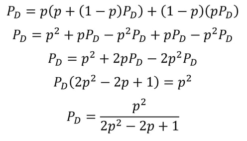 When we graph this equation, we get the following shape: 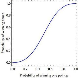 The shape of this graph is quite interesting. When p is 0.5, the probability of winning from deuce is also 0.5, so chances are even. But if p differs even slightly from 0.5, the chances of winning from deuce increase or decrease quite significantly. The shape of this graph demonstrates that players need to have very similar point probabilities for a game to be close. Given that so many matches in today's climate are very close, this shows just how close to each other the players are in ability, and how even a slight edge can have huge consequences.
Let us know in the comments if you were interested in this article about maths in sports, and tell us what you'd like to read about next! Malhar Rajpal Most math competitions have stringent time limits and a prohibition of calculator use. Because of this, it is extremely important to learn basic strategies to perform quick mental calculations to solve more problems and thus be more successful in such competitions. Furthermore, performing mental math in front of a live audience is extremely impressive: imagine squaring huge numbers in your head quicker than any calculator can do it! In this article, you will learn the strategy of quickly squaring two digit numbers and the reasoning behind the method.
Squaring a two digit number in your head: Imagine seeing 56x56 on your exam paper, as you’re scramming for time. It would be a huge pain to calculate this using table multiplication and you would save at least half a minute by doing this in your head. How would we do this? The method: If we take any two digit number, say in this case we take 56, we first round it to the nearest 10. So if our number is 56, we round to 60. If our number is 42, we would round to 40. Then you find the difference between the rounded value and the initial value. So 60-56 = 4 or 42-40 = 2 and you perform the “reverse calculation” by that same value: If you initially chose 56, you have to add 4 to get 60, and hence the reverse calculation would be to subtract 4, and this number would be 56-4 = 52. If you had to square 42, you subtract 2 to get 40, and hence the reverse calculation would be to add 2 to get 42+2 = 44. After you get the two numbers, the rounded number and the number you obtained after performing the reverse calculation, you multiply them together. So for squaring 56, you would multiply 60 and 52, which is just 6x10x52 = (6x52)x10 = 3120 and for squaring 42, you would multiple 40 and 44, which is 4x10x44 = (4x44)x(10) = 1760. After you have this number, you take the difference between the rounded number and the initial value that you found before and square it. So for 56, 60 is the number rounded to the nearest 10 and 60-56 = 4. We take 4 and square it to get 16. For 42, 42-40 = 2, so we take 2 and square it to get 4. After we get this squared value, we add it to the product that we calculated(the product after multiplying the rounded number and the reverse calculation number). So for 56, we have 3120+16 = 3136, and for 42, we have 1760+4 = 1764, which are our final answers! Amazing how simple it is, isn’t it! It’s simpler than trying to do it manually because you are essentially multiplying a two digit number with a multiple of 10(which is the same as multiplying a two digit number by a one digit number and then multiplying the product by 10), and then adding a small number to that result to get the final answer. Let’s try one more example: 73. 73 rounded to the nearest 10 is 70. 73-3 = 70, hence the reverse calculation is to add 3 to 73: 73+3 = 76. We then multiply 76 with 70 which is the same as 76x7x10 = 532x10 = 5320. The difference between the rounded number, 70, and initial number to square, 73 is 3, and 3 squared = 9. We, thus, add 9 to our existing product to get: 73x73 = 5320 + 9 = 5329, our final answer! The mathematics and reasoning behind the method: The mathematics behind this method is actually very simple. Let’s say we have a number, a. We want to find a^2. By the method, we are adding or subtracting some value b from a to get the rounded value. We then perform the reverse operation subtracting or adding b from a. Finally we multiply these two numbers together and this can be represented as: (a+b)(a-b) where the first number is the rounded up value, and the second number is the number after performing the reverse operation on a. We could also have (a-b)(a+b)if the rounded number is rounded down instead of up, however, since xy =yx, (a+b)(a-b)=(a-b)(a+b) hence both expressions are equivalent. After we evaluate the product (a-b)(a+b), we add the value of b^2 to the product to obtain our final answer. We can thus hypothesise that a^2=(a-b)(a+b) + b^2 and now we have to prove this. The proof is direct and just requires an expansion of the right side: a^2=a^2-b^2+b2 and the b^2s cancel out leaving us with a^2=a^2, an equivalent statement so we know that a^2=(a-b)(a+b)+b^2 is true and our methodology therefore works for any real a and b! Nitya Nigam Since the advent of modern computing in the 1950s, computers have played an essential role in mathematical research. They're often used to test conjectures, as they can iterate through long lists of numbers extremely quickly to check whether they satisfy the conditions that have been predicted. They are also used to find specific types of numbers, such as Mersenne primes (you can even join the Great Internet Mersenne Prime Search yourself). However, coming up with conjectures has long been the work of mathematicians themselves. A good mathematical conjecture states something profound and useful within the field. It must be interesting enough to prompt investigation, but not so niche as to have very narrow applications. Getting computers to strike this balance is therefore a tall task.
However, researchers at the Technion in Israel have created an automated conjecturing system called the Ramanujan Machine, named after the famous mathematician Srinivasa Ramanujan. The software has already conjectured original formulas for several mathematical constants (published in this Nature article) including Catalan's number and pi. The software works by leveraging the fact that many such constants are equal to continued fractions (fractions where the denominator is the sum of two terms, one of which is a fraction with a denominator that also contains a fraction, and so on until infinity). Continued fractions have been of mathematical interest both for their aesthetics and what they reveal about constants' fundamental properties. The software works by first finding continued fraction expressions that seem to equal universal constants by choosing arbitrary constants and expressions, then computing each side to a certain level of precision and seeing if they approach each other. If they seem to approach each other, they are computed to higher precision to ensure that it is not a coincidence. Since formulas already exist to compute pi and other constants to an arbitrary level of precision, the only thing in the way of making sure the sides match is computing time. So far, the software has conjectured a formula for Catalan's constant that allows for its fastest computation yet. This is an important milestone for computational mathematics, not just because it shows promise for developing faster methods to compute other constants, but because these automated conjectures may be used to reverse-engineer more theorems, further fueling mathematical innovation, Malhar Rajpal In physics, a capacitor is a device that stores electrical energy. A capacitor is made up of two plates with a dielectric material between the plates. When a voltage is applied to a circuit with a capacitor, positive charge builds up on one plate while negative charge builds up on another plate, with the result being a potential difference (potential refers to the electrical potential as a result of the different charge between the plates). When the potential difference of the capacitor is the same as the voltage applied in the circuit, the current in the circuit becomes 0 and the capacitor’s p.d. stops increasing. The ‘charging’ process for the capacitor happens very quickly when there is no resistance in the circuit. If there is a resistance, by I=V/R, the current is lower and thus the charge builds up slower on the plates, slowing down the charging process. The more resistance, the slower the capacitor reaches the voltage applied. A capacitor also has a property called capacitance, C, which is the ratio of the amount of electric charge stored on a conductor to the difference in electric potential (this is directly proportional to the area of the plates and inversely proportional to the distance between the plates). The maximum charge on a capacitor is given by the equation Q = CV, where Q is charge, C is capacitance, and V is voltage. The capacitor can then be removed from the circuit with the power source and put in another circuit without a power supply. The charge then dissipates from the capacitor and flows through the circuit. This causes the absolute value of the charges on the plates and therefore the potential difference to decrease until they reach 0. The rate that the charge decreases with time of some capacitor with capacitance C depends on the resistance of the circuit and today we will explore the mathematical model finding the charge Q in this circuit at any given time while the charge dissipates. In the new loop, with the capacitor and some resistance, R, the current I of the circuit can be modelled by: I=V/R and V=IR. From above, we have the equation linking charge to capacitance and p.d.: Q = CV. Rearranging this equation, we see that V = Q/C. Substituting V = IR, IR = Q/C and thus I=Q/(RC). Current is also defined as the net rate of flow of electric charge, which can be defined mathematically as the change in charge over the change in time: ΔQ/Δt. Since charge is being dissipated (decreasing), we can say that ΔQ/Δt must be negative and, being physicists (this step is illegal is maths!), we can can say that I = -ΔQ/Δt. Now that we have two expressions for I, we can combine them: -ΔQ/Δt = Q/(RC), a differential equation! Using calculus notation, -dQ/dt=Q/(RC). Rearranging this equation, we get (1/Q)dQ = -1/(RC) dt. We can now integrate both sides: 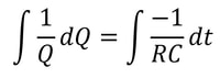 Since we don’t want the unknown constants resulting from indefinite integration in our final expression, we need to make both integrals definite (along a fixed range). We can say that we start at t=0 and go until t=t. When t=0 seconds, Q = Q_0 (initial capacitance), and when t=t seconds, we can say that Q=Q (some capacitance). So we get: 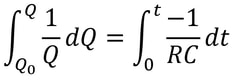 Solving this, since -1/(RC) is a constant with respect to t, we can bring it out of the integral to get: 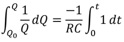 The indefinite integral of 1/Q dQ is just ln(Q) + C (natural log of Q), where C is an arbitrary constant, so by using the definite integrals, the left side of the equation is: 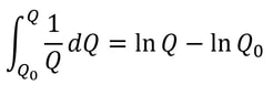 The indefinite integral of dt is just t+c and thus the right side becomes: 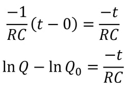 Using ln(a) - ln(b) = ln(a/b), ln(Q) - ln(Q_0) = ln(Q/Q_0). We can now raise e (Euler’s constant) to the power of both sides to get: 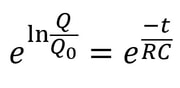 Since e^(ln(a)) = a for any a, we can rewrite as Q/Q_0= e^(-t/(RC)) and thus: 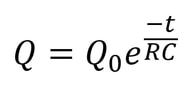 where Q is charge, Q_0 is initial charge, e is Euler’s constant, t is time since discharge begun, R is resistance, and C is capacitance.
The units of RC is seconds and it is thus be referred to as the time constant, τ. Using Q=Q_0 e^(-t/(RC)), when t = τ, Q = Q_0/e; when t = 2τ, Q = Q_0/e^2; when t = 3τ, Q = Q_0/e^3. In every discharge cycle, the time constant is equal to the amount of time taken for the charge to reduce to ~37% (1/e) of its initial value. Since charge is easily measured and this time is a constant, one great use for capacitors is in timing circuits! As an exercise for yourself, try showing that the equations V=V_0 e^(-t/(RC)) and I = (V_0 / R) e^(-t/(RC)) also hold true in RC circuits! Nitya Nigam Rounding numbers is a concept you were probably taught in primary school. The rule generally told to 7-year-olds is that numbers ending in 1-4 are rounded down, while numbers ending in 5-9 are rounded up (numbers ending in 0 aren’t rounded at all). This is a bit of an arbitrary rule - there are 9 numbers (1-9) that are rounded, and 5 is directly in the middle of them. It could be rounded either up or down, but convention states it should be rounded up, so we do. However, consistently rounding 5 up introduces systematic error: an error that is always wrong in a particular direction.
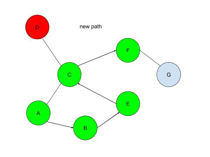
Let’s look at an example. Consider the numbers 0.5, 1.5, 2.5, 3.5, 4.5, 5.5, 6.5, 7.5, 8.5, and 9.5. The average of these numbers is 5. If we were to round all of these numbers as taught, you get 1, 2, 3, 4, 5, 6, 7, 8, 9 and 10. The average of these is 55/10=5.5, which is 0.5 higher than the real average. This means we have an error of 0.5 through this rounding method. A better rounding method for numbers with 5 as their last digit would be to round to the nearest even digit. This gets rid of systematic error as you would be rounding up and down equally often (at least in theory). We can see this clearer through an example. Using the same dataset as above, if we round each number to the nearest even digit, we get 0, 2, 2, 4, 4, 6, 6, 8, 8, 10. The average of this is 50/10=5, meaning we have an error of 0. Although this method of rounding 5s to the nearest even digit helps reduce error (it is actually used quite often in scientific data collection, despite it not being widely known in other contexts), it’s a bit difficult to explain to 7-year-olds. The simplification of always rounding 5 up works well enough for basic applications, but it’s important to keep in mind that it does produce a systematic error. Next time you’re taking data in a science class, try both methods of rounding, and see how much difference there is between the two! Let us know what you find in the comments section. Malhar Rajpal Last week's article outlined the underlying structures of depth first search. Check it out here before continuing with the rest of this article, which will describe how the algorithm actually works! By using the stack data structure, we must explore the last node that was added to the frontier. Since A in the table above is the only node in the frontier, it is also the last node that was added and is therefore explored. By the exploration process mentioned above, the algorithm first checks whether node A is the solution node. Since the program knows that node G is the solution, our algorithm deduces that node A is not the solution node. It, therefore, retrieves all the nodes connected to node A, namely node B and node C. It then checks if either of these nodes are in the explored nodes list. Since neither of them are, the program adds them to the frontier arbitrarily(let’s say C is added before B in this case, however it could also be the other way around). Node B and C also have a link to their parent element, node A stored inside of them. Node A is then removed from the frontier and added to the explored nodes list: 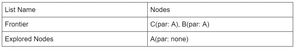 Since B was the last node to be added to the frontier, by the rules of the stack, it is the next node to be explored. By using the same process as above, we see that node B is not the solution node. The nodes directly connected to B, nodes A and E, are retrieved. Since node A is already in the explored nodes list, it is ignored. Node E, which isn’t in the frontier or the explored nodes list is then added to the frontier. Node B is then transferred to the explored nodes list: 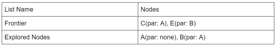 If you follow the same process as above, you should figure out that after exploring node E, no new nodes are added to the frontier(since node C is already in the frontier and node B is already explored). Thus we end up with the table: 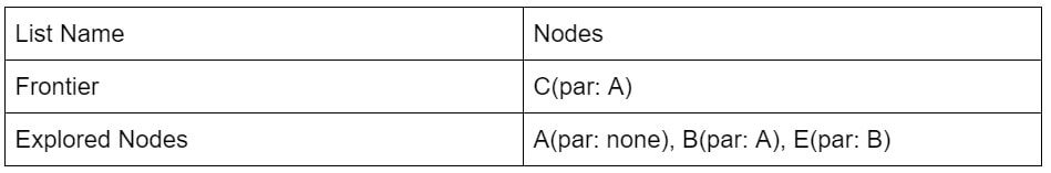 After exploring node C, two new nodes: node F and node D are added to the frontier(let’s assume in the order F then D). The other two nodes that connect with node C: node E and node A are ignored because they have already been explored. However, if you wish to code a more complex algorithm, you could show that since there is at least one explored node between node A and node C, since node C connects with node A, and since node C also directly connects with the previously explored node(E), there is a cycle in the graph. The length of this cycle could also be determined. 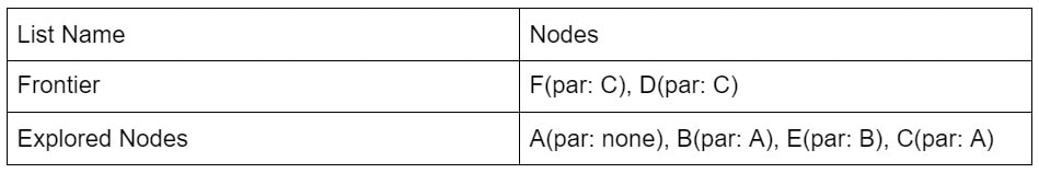 After exploring D, nothing new is added to the frontier. This is because the only node connecting node D is node C which had just been explored. Because of this, node D is classified as a ‘dead-end’. When a DFS algorithm reaches a dead-end, it backtracks to the last decision point and follow the path resulting from another choice:
We see that after DFS sees that node D is a dead-end, it backtracks to the last decision point(node C), and makes the other decision(traversing to node F). This is automatically done through the stack frontier procedure described above. 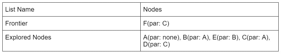 Node F is then explored and it is evident that node G is the only node that is added to the frontier: 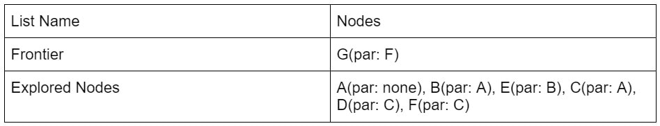 Now our exploration process checks Node G against the solution and it determines that Node G is in fact our goal node! Since we kept track of the parents, we can easily backtrack the optimal route from the solution node(Node G) all the way to the initial Node. We can do this by creating a list and adding the subsequent parent elements of each of the previous nodes to the list, until we reach node A(which has par:none). Hence from Node G, we go to it’s parent, Node F, then to its parent, Node C, and continue until we reach Node A. This gives us this list: (G, F, C, A). Reversing this list, we can find a route to node G: (Node A → Node C → Node F → Node G)!
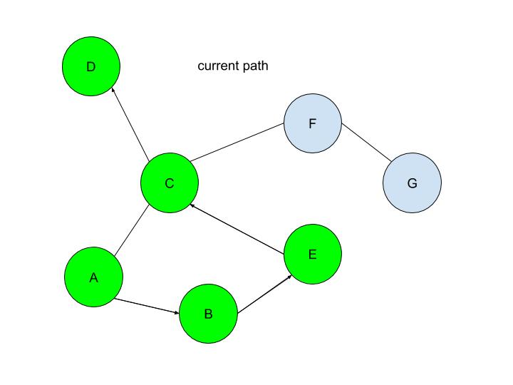
If the problem was more complex, stacks would have ensured that each branch was explored until a dead end was reached(such as node D in this case), before backtracking to the last possible decision point(a node connecting to several other nodes) and exploring another branch from there(by traversing to a different node than it did initially). DFS is a powerful, uninformed search algorithm that can be used in a variety of situations, such as solving single solutioned maze problems, performing topological sorting, and is even used in Minimax, which is shown in one of my previous articles! It also sets the foundation of better, more efficient heuristic functions (such as greedy best first search or A* search which are informed search algorithms). If you have read my article on BFS, you may be wondering, when you should use BFS over DFS, or vice versa. Don’t fret, because in my next article, I will evaluate the strengths and weaknesses of both the algorithms! Malhar Rajpal This is the first of a two-article piece on depth first search. From performing topological sorting to solving puzzles with one solution(such as mazes), depth first search is a powerful search algorithm that can be used to crack a large variety of problems. In any puzzle, for example a maze, depth-first search (DFS) works by exploring one route in its entirety (until a dead-end is reached or the solution is obtained). If the solution is obtained, it returns the correct path. If not, the algorithm is programmed to backtrack and try out another route in its entirety, performing the same process. To perform this, DFS uses a data structure called a stack, which is a last in, first out data type (don’t worry if you don’t understand this yet). The puzzle: To explain the concept of a stack and DFS, I will use an unweighted graph: 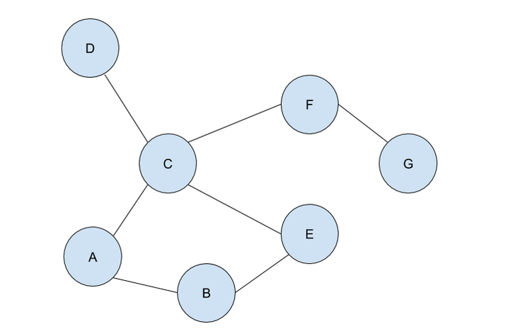 Let’s assume we start at circle A on the unweighted graph and we want to make our way to circle G. We can visualise this as a simple maze, where every line (or edge more formally) that connects two circles (more formally called nodes) is a possible move from one place to the next. Nodes with no edges connecting it except for the one that led to it (such as node D) can be considered as a ‘dead end’. Our goal is to use the DFS algorithm to find the route from starting point, node A, to the end of the maze, node G. Obviously, since this maze is very simple, we can visually see that the answer is A → C → F → G, however we want to know how an algorithm can figure this out, and how this method can be used to solve more complex puzzles that we perhaps couldn’t solve visually. Initialising the algorithm: The DFS algorithm requires a list which is more formally called the frontier. This frontier contains the nodes that are currently being explored or will be explored in the future (unless the solution is reached before the node can be explored). Another list containing the already explored nodes is also needed. When we begin running the algorithm, our initial node A is put into the frontier (shown below), since it is the first node that will be explored. Since no nodes have been explored yet, the list containing the explored nodes remains empty.  Stacks:
The stack data structure used for DFS is a last in, first out data type. Simply put, this means that the frontier will explore and remove the node that was last appended to the frontier list. This explored node then gets transferred to the explored nodes list. But what exactly do we mean by ‘the frontier will explore’ a node? The exploration process: Exploring a node includes checking if the currently explored node is equal to the solution node (in this case node G) or if node ‘solution node’ is explicitly stated, then by checking whether the currently explored node follows all the conditions in a predetermined set of criteria that defines the solution (criteria such as the solution node must be connected to node F and no other node). If it is deduced that the current node is the solution node, then the program can return the path needed to reach the final node. If it is not, then all the nodes that connect with the current node are retrieved. A check is performed on each of the connected nodes: if the node has already been explored (if it’s in the explored nodes list already) and if it’s not already in the frontier, then it is ignored. If it hasn’t been explored, then it will be added to the frontier. The order of the connected nodes being added to the frontier is completely arbitrary in DFS. The node has now been explored and is thus moved from the frontier list to the explored nodes list. The nodes: Each node stores its needed data (whatever it may be) as well as the parent node within itself. For example, Node B contains its own information as well as that of its parent element (Node A). These parents will be labelled in our table using the format ‘par: letter of node’ (appearing in my next article). This is to back-track and find the correct path from the initial position to the solution once the solution node is reached. The parent node of some node is easily found: we can refer to the parent node of some node as the node which was being explored right when this new node was first brought to the frontier. Check out my next article to see how the algorithm works on an example! Nitya Nigam Get your power tools out and start building, because scientists from the University of Queensland in Australia have proven that time travel is theoretically possible after resolving a logical paradox. Germain Tobar and Fabio Costa used mathematical models to align classical dynamics (Newtonian physics) with general relativity (proposed by Einstein). You can find their full paper here, but we’ll be summarising its findings in the rest of this article.
You may have heard of the grandfather paradox, which is a commonly cited logical problem with the concept of time travel. If someone were to go back in time and kill their grandfather, classical dynamics states that the events following the grandfather’s demise would result in the time traveller not being born. However, relativity allows for the time traveller to use a “time loop” (formally called a closed timelike curve, or CTC) to go back in time and kill their grandfather. CTCs are essentially results of solutions to the mathematical equations of relativity. The methods used by Tobar and Costa reconcile this maths with that of classical dynamics. The two scientists used the model of the COVID-19 pandemic to work out whether the two conflicting theories could coexist. What they found is that events would realign themselves so that even if someone went back in time from t=0 and stopped COVID-19 from infecting a human at, say, t=-10000, the end result of the pandemic at t=0 would still occur. “In the coronavirus patient zero example, you might try and stop patient zero from becoming infected, but in doing so you would catch the virus and become patient zero, or someone else would,” explained Mr Tobar. Essentially, regardless of what you did as a time traveller, events would recalibrate themselves without you, meaning that the pandemic would occur and give your original self a reason to go back in time and stop it. Mr Tobar summed this up by saying: “The range of mathematical processes we discovered show that time travel with free will is logically possible in our universe without any paradox.” Dr Fabio Costa added: “The maths checks out - and the results are the stuff of science fiction.” This is truly some remarkable research, but readers must keep in mind that this paper has only been through one round of peer review, so there may be errors in the paper that haven’t been caught just yet. Furthermore, this only shows that there is a possibility for logically consistent time travel, not that this definitely can exist. But this is definitely a win for all the sci-fi nerds out there. |