|
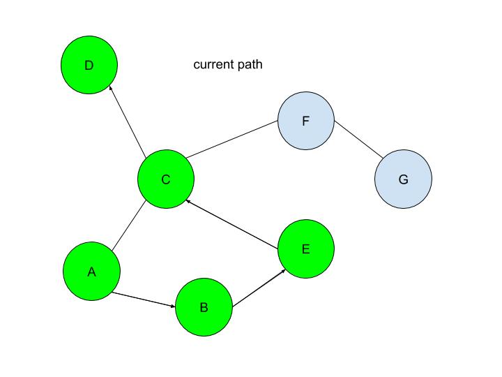
Malhar Rajpal Last week's article outlined the underlying structures of depth first search. Check it out here before continuing with the rest of this article, which will describe how the algorithm actually works! By using the stack data structure, we must explore the last node that was added to the frontier. Since A in the table above is the only node in the frontier, it is also the last node that was added and is therefore explored. By the exploration process mentioned above, the algorithm first checks whether node A is the solution node. Since the program knows that node G is the solution, our algorithm deduces that node A is not the solution node. It, therefore, retrieves all the nodes connected to node A, namely node B and node C. It then checks if either of these nodes are in the explored nodes list. Since neither of them are, the program adds them to the frontier arbitrarily(let’s say C is added before B in this case, however it could also be the other way around). Node B and C also have a link to their parent element, node A stored inside of them. Node A is then removed from the frontier and added to the explored nodes list: 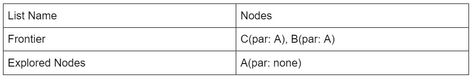 Since B was the last node to be added to the frontier, by the rules of the stack, it is the next node to be explored. By using the same process as above, we see that node B is not the solution node. The nodes directly connected to B, nodes A and E, are retrieved. Since node A is already in the explored nodes list, it is ignored. Node E, which isn’t in the frontier or the explored nodes list is then added to the frontier. Node B is then transferred to the explored nodes list: 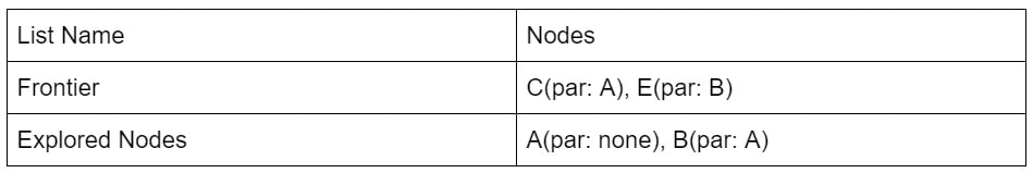 If you follow the same process as above, you should figure out that after exploring node E, no new nodes are added to the frontier(since node C is already in the frontier and node B is already explored). Thus we end up with the table: 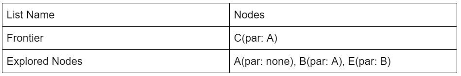 After exploring node C, two new nodes: node F and node D are added to the frontier(let’s assume in the order F then D). The other two nodes that connect with node C: node E and node A are ignored because they have already been explored. However, if you wish to code a more complex algorithm, you could show that since there is at least one explored node between node A and node C, since node C connects with node A, and since node C also directly connects with the previously explored node(E), there is a cycle in the graph. The length of this cycle could also be determined. 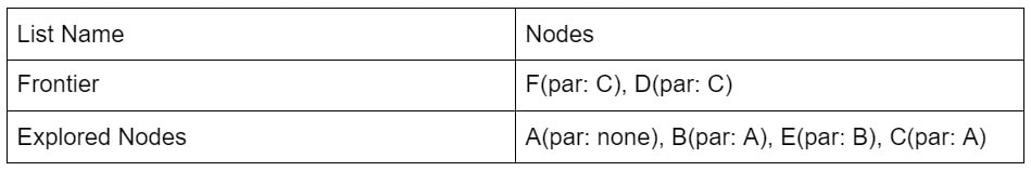 After exploring D, nothing new is added to the frontier. This is because the only node connecting node D is node C which had just been explored. Because of this, node D is classified as a ‘dead-end’. When a DFS algorithm reaches a dead-end, it backtracks to the last decision point and follow the path resulting from another choice:
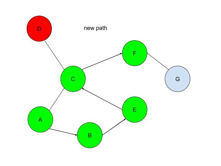
We see that after DFS sees that node D is a dead-end, it backtracks to the last decision point(node C), and makes the other decision(traversing to node F). This is automatically done through the stack frontier procedure described above. 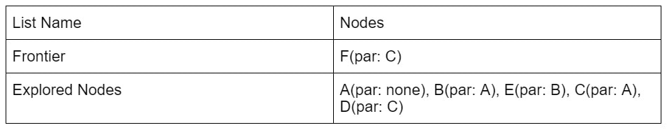 Node F is then explored and it is evident that node G is the only node that is added to the frontier: 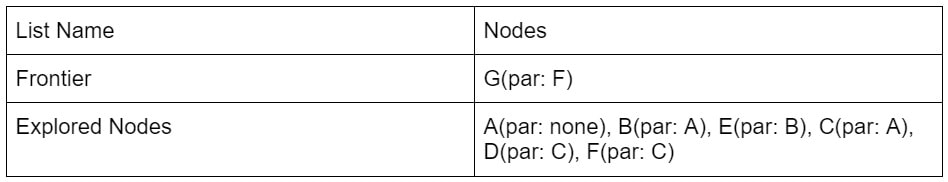 Now our exploration process checks Node G against the solution and it determines that Node G is in fact our goal node! Since we kept track of the parents, we can easily backtrack the optimal route from the solution node(Node G) all the way to the initial Node. We can do this by creating a list and adding the subsequent parent elements of each of the previous nodes to the list, until we reach node A(which has par:none). Hence from Node G, we go to it’s parent, Node F, then to its parent, Node C, and continue until we reach Node A. This gives us this list: (G, F, C, A). Reversing this list, we can find a route to node G: (Node A → Node C → Node F → Node G)!
If the problem was more complex, stacks would have ensured that each branch was explored until a dead end was reached(such as node D in this case), before backtracking to the last possible decision point(a node connecting to several other nodes) and exploring another branch from there(by traversing to a different node than it did initially). DFS is a powerful, uninformed search algorithm that can be used in a variety of situations, such as solving single solutioned maze problems, performing topological sorting, and is even used in Minimax, which is shown in one of my previous articles! It also sets the foundation of better, more efficient heuristic functions (such as greedy best first search or A* search which are informed search algorithms). If you have read my article on BFS, you may be wondering, when you should use BFS over DFS, or vice versa. Don’t fret, because in my next article, I will evaluate the strengths and weaknesses of both the algorithms!
0 Comments
Leave a Reply. |