|
Malhar Rajpal The quadratic formula is used by most secondary students to solve quadratic equations in the form ax^2 + bx + c = 0. But most of these students don’t know where the formula comes from. In this article, I will explain the derivation of the quadratic formula. The idea of the quadratic formula is to isolate x from the initial equation, ax^2 + bx + c = 0. We can subtract c from both sides of the equation to get ax^2 + bx = -c. We then proceed by dividing both sides by the coefficient of x^2, namely a: 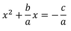 The next step requires some creativity since these steps are unintuitive and rather inventive. Firstly, we must identify the coefficient of the linear (x) term in the above equation. This is b/a. We then divide this term by 2 and square it to get: (b/2a)^2=(b^2)/(4a^2). We add this term to both sides of the above equation to get: 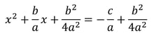 That was the creative step. We can now simplify the equation by making the terms on the RHS of the same denominator, and by completing the square on the LHS: 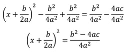 We now take the square root of both sides: 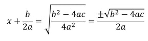 Finally we subtract b/2a from both sides to get the quadratic formula: 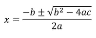 Now you know how to derive the quadratic formula, you can use it in a classroom situation without worrying whether it actually makes sense!
0 Comments
Nitya Nigam 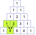 Pascal's triangle, as many of you may already know, is a mathematical pattern where the nth row is the sum of nCk from k=0 to k=n. As shown in the diagram on the left, each number is obtained by adding together the two numbers directly above it. In this article, we will investigate some of the patterns hidden in Pascal's triangle. As mentioned in the solution to May 24th's problem of the week, the sum of nCk from k=0 to k=n is 2^n, which means that the sum of rows in Pascal's triangle is 2^n. We can prove this quite easily using the binomial theorem. The binomial theorem states that:  Letting x=y=1: 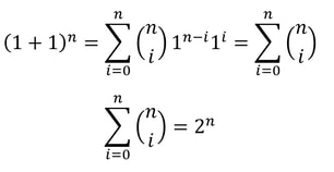 which proves our claim. Another interesting pattern in the triangle is that the squares of the numbers on the second diagonal are equal to the sum of the two numbers directly next to and below it, as shown in the diagram below: 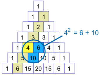 To prove this, we need to recognise that the third diagonal is the triangular numbers, which have formula n(n+1)/2. The sum of two consecutive triangular numbers is: 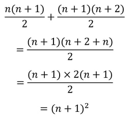 which is the necessary square number.
Pascal's triangle is full of many more interesting patterns - let us know in the comments what you'd like to learn about next! Malhar Rajpal Most high school students will have heard of the infinite geometric series formula as well as the sum of an arithmetic sequence formula. Most of us just accept these blindly without an explanation as to why they truly work. However, today we will prove both the formulas infinite and finite geometric series sums as well as the formula for the sum of an arithmetic sequence! For those who haven’t encountered these terms before, an arithmetic sequence is a sequence of numbers such that the difference between consecutive terms is constant. The nth sum of an arithmetic progression is thus the sum of all the numbers in the sequence up to the nth term of the sequence. Evidently, since the difference between consecutive terms is constant, the numbers will eventually be either very large and positive or very low and negative and the infinite sum of an arithmetic sequence is thus divergent. An infinite geometric series is the sum of an infinite number of terms in a sequence wherein there is a constant ratio between successive terms (sum of infinite values in a geometric sequence). It is important to note than an infinite geometric series only converges if the absolute value of the common ratio r is less than 1. As the name suggests, a finite geometric series is the sum of a finite number of terms (up to the denoted nth term) of a geometric sequence. Arithmetic Series formula proof: The formula for an arithmetic series, adding up each of the first n terms of an arithmetic progression is given by: 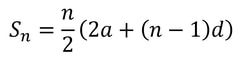 where S_n the sum of the first n terms of an arithmetic sequence, a is the first term of the sequence, n is the number of terms we want in the sum, and d is the common difference between successive terms in the arithmetic sequence. To prove this formula, we must first look at the base definition of an arithmetic series which is adding up the first n terms of an arithmetic sequence: S_n=a+(a+d)+(a+2d)+(a+3d)+...+(a+(n-2)d)+(a+(n-1)d), or Sn=(a+(n-1)d)+(a+(n-2)d)+...+(a+3d)+(a+2d)+(a+d)+a (which is the same as above but backwards. If we add the first term of the first S_n formula with the first term of the second S_n formula, and the second term of the first S_n formula with the second term of the second Sn formula, and so on, we see that each term adds up to 2a+(n-1)d: For example: a+(a+(n-1)d) = 2a+(n-1)d and (a+d)+(a+(n-2)d) = 2a+(n-1)d… Hence by adding both the S_n together, we get: 2S_n=(2a+(n-1)d)+(2a+(n-1)d)+...+(2a+(n-1)d) Since we are adding the first n terms of the arithmetic sequence, there are thus n occurrences of 2a+(n-1)d in the formula for 2S_n. Thus: 2S_n=n(2a+(n-1)d) And by dividing two from both sides, we reach our desired formula: S_n=(n/2)(2a+(n-1)d) And the arithmetic series formula is proven. Finite Geometric Series Proof: The formula for the sum of a finite geometric series is: 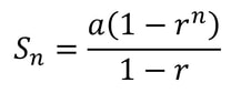 where S_n in this case denotes the sum of the first n terms of a geometric sequence. r is the common ratio between consecutive terms and n is the number of terms we want to sum. To prove this formula, let’s look at the defining formula for a finite geometric sequence, which includes summing up the n terms of the sequence: Sn=a+ar+ar^2+...+ar^(n-2)+ar^(n-1) We can create another formula by multiplying each term by r: rSn=ar+ar^2+....+ar^(n-2)+ar^(n-1)+ar^n The difference between these two formulas is that the formula for S_n has the term a while the formula for rS_n has the term ar^n. Both the formulas have all the other terms, ar+ar^2+...+ar^(n-1). Because of this, we can subtract rS_n from S_n to get: S_n-rS_n=a-ar^n. Factoring out both sides: S_n(1-r)=a(1-r^n) Dividing both sides by 1-r (which is possible since we don’t consider r=1 in this case) to get our desired formula: S_n=a(1-rn)/(1-r) , r≠1 And we have proven the formula for a finite geometric series! Infinite Geometric Series Proof: The textbook formula for the sum of an infinite geometric series is: S_∞=a/(1-r), -1<r<1 To determine the proof, we can evaluate the S_n formula for a finite geometric series as n tends to ∞. We thus get: 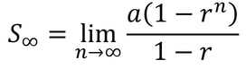 The limit can only be solved if -1<r<1 since if r doesn’t fall within this range, the r^n term diverges as n tends to ∞. However, if r falls within the range -1<r<1, as n approaches ∞, the r^n term approaches 0. Thus we get our desired formula: 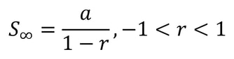 And the final formula for this article is proven!
Nitya Nigam Graph theory is having a great year. Following the proof of lower bounds on Ramsey numbers (link is to our coverage) from Asaf Ferber and David Conlon in late 2020, a new proof has proved a special case of the Erdős-Hajnal conjecture. Essentially, the conjecture implies that forbidding certain structures at a small scale impacts the macroscopic structure of the graph, which has powerful consequences for graph theory (we'll go into more detail later in the article). The new proof, published in February by Maria Chudnovsky and Paul Seymour of Princeton University, Alex Scott of the University of Oxford, and Sophie Spirkl of the University of Waterloo, proves two special cases of the conjecture, so although a complete proof still evades us, significant progress is being made. More formally, the Erdős–Hajnal conjecture states that if a graph does not contain a certain structure (known as an induced subgraph), then the graph will inevitably have either a large clique or a large independent set. Let's define these terms: Clique: A subset of vertices in a graph such that every vertex is connected to every other member of the subset via at least one edge. Independent set: A subset of vertices in a graph such that every vertex in the subset is not connected to any of the other vertices in the subset. Large: A large clique or independent set in a certain graph with V vertices is defined as a clique or independent set with more vertices than would arise if a random graph with V vertices was drawn. 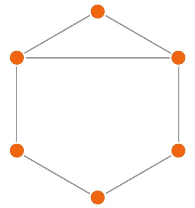 Chudnovsky and her colleagues proved the conjecture for two special cases. One was the specific forbidden induced subgraph of a "five-cycle" - a set of 5 vertices where each vertex is connected to exactly two others in the set. The other was a "five-cycle with a hat" - a set of 6 vertices similar to a 6-cycle, but with an extra edge joining two vertices (shown on the left). While most conjectures are formed with mathematical consensus agreeing they are likely to be true, the mathematicians working on this problem actually expected that they would disprove the conjecture: that is, that it would be false. “We were all a little shocked,” said Chudnovsky. Prior to this paper, the conjecture had only been proven true for induced subgraphs of four vertices or fewer, as well as another special 5-vertex subgraph ("The Bull" below) by Chudnvosky and Shmuel Safra in 2005. 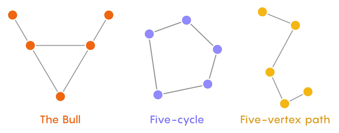 This leaves just the five-vertex path as the last possible five-vertex induced subgraph, and the clear next step for eventually proving the full conjecture. “The five-vertex path has to be next. If you can’t do that, you’re still nowhere,” said Paul Seymour. We're excited to see what developments are still to come!
Malhar Rajpal In my last article, I talked about László Lovász, one of this year’s winners of the prestigious Abel Prize. In this article, I will talk about the background and accomplishments of this year's other recipient, Avi Wigderson.
On 9th September 1956, Avi Wigderson was born in Haifa, Israel. He graduated with a B.Sc. in Computer Science from the Technion (The Israeli Institute of Technology) in 1980. He then went to Princeton University in the USA for his graduate studies, where he completed his PhD in computational complexity under Richard Lipton. Wigderson's major contributions are in the field of computational complexity, which is the study of how quickly computer problems can be solved. You may have heard of the P=NP problem, which is the fundamental question of computational complexity. Computer problems are designated as P (meaning they can be easily solved in polynomial time) or NP (meaning it would take a very long time to solve the problem with known algorithms, but the answer can be verified quickly). Computational complexity is thus founded on the question of whether all the hard to solve problems in the NP set can be reduced to problems that are easy to solve and are in the set P, and thus whether P = NP. This is an unsolved and hotly debated question in mathematics. Wigderson made remarkable developments in this field. One of his biggest achievements is researching how randomness can be used to solve computational problems in a quicker period of time. He showed that if a computer can “flip coins” during the computational process, rather than if the computer chooses each decision, then a solution to a computational problem can be reached in a quicker period of time. This was massive, and it showed that randomness could be used to facilitate a great deal of tasks in the computational world. Dealing with randomness, however, increases the chance of an error in the solution, and therefore Wigderson, with Noam Nisan and Russell Impagliazzo, showed that for any algorithm that uses coin flipping to solve a difficult problem, there is another algorithm that is nearly as fast that uses deterministic (non-random) methods to reach the same solution, under certain conditions. This finding was a huge accomplishment, as it proved that the problem class known as “BPP” in the computer science world was actually the same as the complexity class P, revolutionising the way random algorithms were perceived. Perhaps what Wigderson is most famous for is his co-discovery of the zig-zag product in 2000. The zig-zag product is an innovative finding that links several different fields such as group theory, graph theory, and complexity theory. Very simply put, the zig-zag product of regular graphs is when one takes a large graph and a smaller graph and produces a new graph with the approximate size of the large graph but the degree of the smaller one. According to Wikipedia, it is “a method of combining smaller graphs to produce larger ones used in the construction of expander graphs”. There are, of course, several intricacies to this finding, however they are beyond the scope of this article. The zig-zag product is extremely powerful and carries a huge number of applications, such as finding the optimal way to solve a maze problem. Although he has co-authored over 100 research papers, it would be impossible to cover all of his brilliant ideas in one article. Nonetheless, these achievements alone are truly extraordinary. Nitya Nigam As promised in March 22nd’s Problem of the Week (apologies for the delay, it’s been a busy month), this is an article explaining the connection between choose functions and polynomial functions. More specifically, we’re going to prove why sequences of the form T_n = nCk (where k is a constant integer) are equivalent to specific polynomial sequences of degree k, as well as find the specific polynomial sequence that fits our POTW. While we will be showing this algebraically, there is also a very interesting analogy to Pascal’s Triangle that shows this, which we’ll leave to our readers to think about (and share their ideas about in the comments!) The example used in our POTW was T_n = nC3 for n≥3. The first few terms of this sequence are 3C3=1,4C3=4, 5C3=10, 6C3=20. We can observe that the differences between consecutive terms (what we call the “first difference”) are 1, 3, 6, 10. While some of you may already have noticed that this sequence is the triangle number sequence, we can go a step further, observing that the difference between these differences (the second differences) are 2, 3, 4 so the third difference is constant at 1. When a sequence has its kth difference constant, the sequence can be written as a polynomial. We can prove this using basic calculus. Say we have a polynomial sequence of the following form: 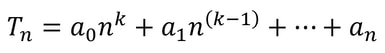 When we differentiate this, the constant term disappears, and the powers on the rest of the terms decrease by 1, giving: 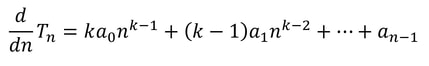 When we differentiate this k times, we get: 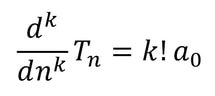 As this expression doesn’t contain any n terms, the kth derivative of a kth-degree polynomial sequence is constant. As the kth difference is simply the rate of change between integer terms, and the kth derivative is the rate of change in general (which is independent of the value of n, so will apply to integers), the two are equal. Therefore, we have shown that the kth difference of a polynomial sequence is constant, and that it is equal to k! times the coefficient on the n^k term. In our example, the third (or kth, as k=3) difference is 1. Since k! x a_0 = 1, a_0 = 1 / k! = 1 / (3x2) = 1/6. Now that we have the leading coefficient, we can simply use simultaneous equations (by plugging in the first three values of n [3, 4, 5]) to obtain the other coefficients. 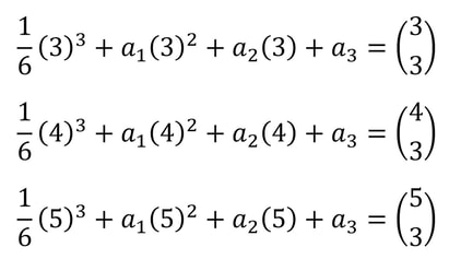 We’ll leave the process of simplifying and solving these equations to you (or your graphic calculator). The result you should get is a_1 = -1/2, a_2 = 0 and a_3 = 1/3, giving the following definition: 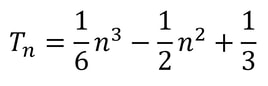 After showing this analytically for the case k=3, let’s generalise. Sequences of the form nCk can be written, from their definition, as: 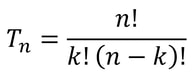 The first difference of these sequences will be T_(n+1) – T_n: 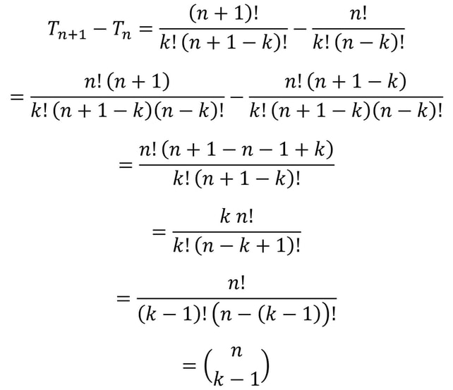 Now, if we’ve shown that the first difference of a sequence nCk is nC(k-1), then by extending this downwards by applying the same thing to the first difference sequence, we can say that the second difference is nC(k-2), and the kth difference is nC(k-k) = nC0, which is just 1. Since the kth difference is constant (which is the condition for a kth-degree polynomial sequence), these sequences can be written as polynomial sequences using the technique described above.
We hope you enjoyed this article, especially since it contained original mathematical ideas from us! Let us know in the comments if you see the link to Pascal’s Triangle, and tell us what you’d like to read next! Malhar Rajpal A few weeks ago, two extremely renowned mathematicians, Avi Wigderson and László Lovász, won the prestigious Abel Prize. Becoming an Abel Prize laureate is not an easy feat, since it is only awarded to the most accomplished mathematicians in a given year. Known colloquially as the Nobel Prize pf mathematics, it has a substantial cash prize of 7.5 million Norwegian Kroner. In this article, I will talk about one of the 2021 Abel Prize winners, László Lovász and his work.
On March 9, 1948, Lovász was born in Budapest, Hungary. He was an extremely talented mathematician from an early age and managed to win three gold medals and a silver medal at the renowned International Mathematical Olympiad, the most competitive and largest high school math competition in the world, where countries send teams of their six best mathematicians to compete. Winning a medal is not an easy feat with only around the top 8% of already brilliant participants receiving a gold medal. Achieving four medals, thus, is quite an amazing achievement and truly showed Lovász’s outstanding mathematical ability at a young age. As a prodigious mathematician, he had the opportunity to meet and learn about game theory from Paul Erdös in his youth. After studying mathematics at the undergraduate and postgraduate level at Hungary's top universities, Lovász became increasingly prominent as a researcher in the field of mathematics and computer science. He worked under the supervision of Tibor Gallai through his doctoral research in the 1970s. He also worked closely with Erdös to develop methods to complement Erdös’ graph theory techniques. One of his largest accomplishments was developing the Lovász local lemma in graph theory which states that as long as a certain number of events are ‘mostly’ independent from each other, and aren’t individually very likely, then there will be a probability that none of them occurs. Of course, there are several intricacies to this lemma that are beyond the scope of this article but it was a vital development because it led to breakthroughs in creating existential proofs for rare graphs and is used in the probabilistic method. Relating to graph theory, he also contributed to the formulation of the Erdös-Faber-Lovász conjecture in 1972 which stated that ‘If k complete graphs, each having exactly k vertices, have the property that every pair of complete graphs has at most one shared vertex, then the union of the graphs can be properly colored with k colors’. This conjecture remains unsolved, however, in 2021, a proof of the conjecture was made for all sufficiently large values of k by a team of five researchers. He also proved Kneser’s conjecture in 1978, where Martin Kneser conjectured in 1955 that the chromatic number (the minimum number of colours needed to colour the nodes of a graph such that no two nodes that share an edge have the same colour) of the Kneser graph K(n, k), for n >= 2k is exactly n-2k+2. Lovász proved it by using topological methods which was significant because it made developments to the huge field of topological combinatorics. Further, in 1982, Lovász worked with Arjen Lenstra and Hendrik Lenstra to create the LLL algorithm which is a polynomial time reduction algorithm. This algorithm was a huge breakthrough for Lovász since it led to massive developments in cryptography and polynomial factorisation, the basis of RSA cryptography. This is, by no means, an exhaustive list of Lovász’s numerous accomplishments, and Lovász has made a considerable impact in the fields of mathematics and computer science over the last five decades. He has been rewarded with several prestigious awards and has worked in numerous outstanding institutions including Yale University, Microsoft Research Center, and the Hungarian Academy of Sciences. His Abel Prize for significant contributions to theoretical computer science and discrete mathematics is therefore fully deserved. Nitya Nigam Since the advent of modern computing in the 1950s, computers have played an essential role in mathematical research. They're often used to test conjectures, as they can iterate through long lists of numbers extremely quickly to check whether they satisfy the conditions that have been predicted. They are also used to find specific types of numbers, such as Mersenne primes (you can even join the Great Internet Mersenne Prime Search yourself). However, coming up with conjectures has long been the work of mathematicians themselves. A good mathematical conjecture states something profound and useful within the field. It must be interesting enough to prompt investigation, but not so niche as to have very narrow applications. Getting computers to strike this balance is therefore a tall task.
However, researchers at the Technion in Israel have created an automated conjecturing system called the Ramanujan Machine, named after the famous mathematician Srinivasa Ramanujan. The software has already conjectured original formulas for several mathematical constants (published in this Nature article) including Catalan's number and pi. The software works by leveraging the fact that many such constants are equal to continued fractions (fractions where the denominator is the sum of two terms, one of which is a fraction with a denominator that also contains a fraction, and so on until infinity). Continued fractions have been of mathematical interest both for their aesthetics and what they reveal about constants' fundamental properties. The software works by first finding continued fraction expressions that seem to equal universal constants by choosing arbitrary constants and expressions, then computing each side to a certain level of precision and seeing if they approach each other. If they seem to approach each other, they are computed to higher precision to ensure that it is not a coincidence. Since formulas already exist to compute pi and other constants to an arbitrary level of precision, the only thing in the way of making sure the sides match is computing time. So far, the software has conjectured a formula for Catalan's constant that allows for its fastest computation yet. This is an important milestone for computational mathematics, not just because it shows promise for developing faster methods to compute other constants, but because these automated conjectures may be used to reverse-engineer more theorems, further fueling mathematical innovation, Malhar Rapal While studying for a math competition, I encountered Brahmagupta’s formula, which states that the area of any cyclic quadrilateral (all vertices of the quadrilateral lie on a single circle) is equal to: 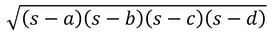 where a, b, c, and d are the 4 side lengths of the quadrilateral and s is the quadrilateral’s semi-perimeter: (a + b + c + d)/2en.wikipedia.org/wiki/Heron%27s_formula. I was astounded by its similarity to Heron's Formula for triangles as well as Bretschneider's formula and wondered why Brahmagupta’s formula stood true for all cyclic quadrilaterals. In this article, I will derive Brahmagupta’s famous formula. 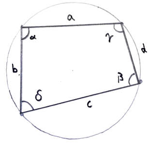 Note: All angles in this article will be referred to in degrees. The diagram above depicts a cyclic quadrilateral with sides a, b, c, d and angles α, β, γ, and 𝛿. One property of cyclic quadrilaterals is that all opposite angles are supplementary. This means that α + β = 180, and γ + 𝛿 = 180. Using α + β = 180, we see that α = 180 - β and thus by apply cosine on both sides: cos(α)=cos(180-β). The difference formula for cosine states that cos(a-b) = cos(a)cos(b) + sin(a)sin(b) for any a and b. We can use this formula on cos(180-β)to get: cos(α) = cos(180)cos(β) + sin(180)sin(β). cos(180)= -1 and sin(180)=0 hence cos(α) = -cos(β). We also apply sine to both sides to get sin(α)=sin(180-β). The difference formula for sine is sin(a-b) = sin(a)cos(b) - sin(b)cos(a) hence sin(α)=sin(180)cos(β)-cos(180)sin(β). sin(180) = 0 and cos(180) = -1, hence sin(α)=sin(β). 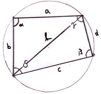 Now, we can split the cyclic quadrilateral into two triangles as shown above with a diagonal of length L. We can use cosine rule for triangles which states that a^2=b^2+c^2 - 2bc cos(A) for triangles with side lengths a, b, c and an angle A opposite to side a. One triangle is bounded by sides a, b, and L and the other triangle is bounded by c, d, L. By applying the cosine rule on both of these triangles, we can see that L^2=a^2+b^2-2abcos(α)and L^2=c^2+d^2-2cdcos(β). We can therefore state that for this cyclic quadrilateral, a^2+b^2-2abcos(α) = c^2+d^2-2cdcos(β) Since cos(α)=-cos(β), we can say that cos(β) = -cos(α). By replacing the occurrence of cos(β) with -cos(α) in the equation a^2+b^2-2abcos(α) = c^2+d^2-2cdcos(β), we get: a^2+b^2-2abcos(α) = c^2+d^2+2cdcos(α) . And by simple rearrangement and factoring: a^2+b^2-c^2-d^2=2cos(α)(ab+cd). Now, we can use the area of the two triangles to get the area of the entire cyclic quadrilateral. Since Area = 1/2 ab sin(C)for a triangle with sides a, b and angle C opposite to the third side (side that’s not a or b), we can see that the area of the triangle bounded by a, b, and L is 1/2 ab sin(α) and the area of the triangle bounded by c, d, and L is 1/2 cd sin(β) . Since the entire cyclic quadrilateral is composed from these two triangles, the area of the quadrilateral is the sum of the areas of the two triangles. Thus, we state that A = 1/2 ab sin(α) + 1/2 cd sin(β). Using sin(α)=sin(β), we replace sin(β) with sin(α)and rearrange to get A=(ab+cd)/2 sin(α) . And by making sin(α) the subject, we get sin(α)=2A/(ab+cd). Brahmagupta faced a problem. How could he relate sin(α)=2A/(ab+cd) with a^2+b^2-c^2-d^2=2cos(α)(ab+cd)? Since for any right angled triangle the sine of an angle is the opposite/hypotenuse and since sin(α)=2A/(ab+cd), the proof creatively formulates a right angled triangle as shown above with hypotenuse ab+cd, a side 2A opposite to an angle α. By using the Pythagorean theorem, the third side becomes: 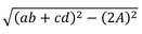 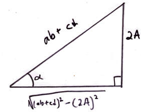 With any right angled triangle, cos(a)= adjacent/hypotenuse. Thus: 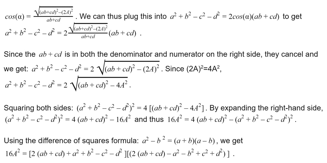 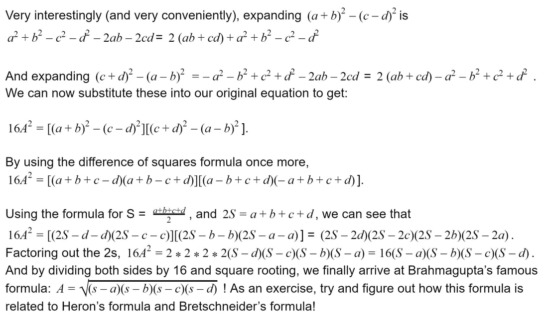 Nitya Nigam A lot of competition maths problems involve finding ratios of areas of various shapes, so having a quick way to find them is a useful tool. In this article, we'll derive the following equation for the area of a regular polygon: 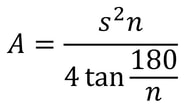 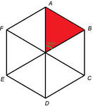 where s is the side length and n is the number of sides. To get to this equation, we first need to consider one of the n triangles that make up the polygon, one of which is shown in red on the right. The central angle of this triangle will be 360/n for any n-sided regular polygon. 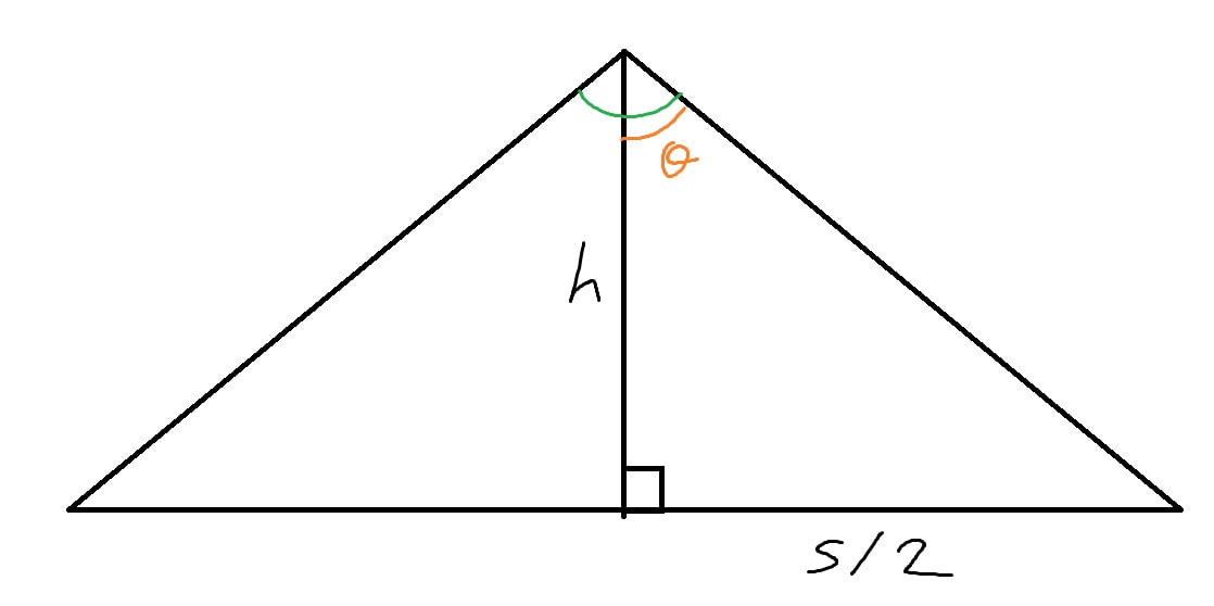 The green angle is 360/n, as stated above, so the orange angle θ is half of that, so θ = 180/n. tan θ = (s/2)/h so h = s / (2 tan θ). The area of a triangle is 1/2 of its base times its height, so the area of this triangle is 1/2 * s * s / (2 tan θ) = s^2 / (4 tan θ). We can then substitute θ = 180/n in, giving A_(triangle) = s^2 / (4 tan (180/n)).
Since there are n of these triangles in an n-sided regular polygon, the total area of the polygon is n * A_(triangle) = n s^2 / (4 tan (180/n)), as above. |