|
Nitya Nigam There are four recognised types of conic sections: circles (probably the most familiar of the lot), ellipses, parabolas and hyperbolas. You’ve probably encountered the equation of a circle: (x-h)^2 + (y-k)^2 = r^2, where (h, k) is the circle’s centre, and r is its radius. In this article, we’ll derive the equations for ellipses and parabolas. Parabolas are defined as curves such that all points on the curve are equidistant from a point, called the focus, and a line, called the directrix. The diagram below displays this clearly: 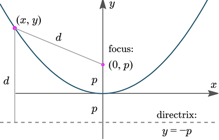 We can see that the vertical distance d from point (x, y) to line y = -p is y + p We can also see that the distance d from point (x, y) to the focus (0, p) is sqrt(x^2 + (y-p)^2) Equating these distances and rearranging gives the following: 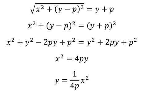 This is the standard equation for a parabola centred at (0, 0). As with the circle equation, we can shift parabolas around by incorporating the parameters (h, k) into the equation like so: 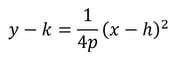 And that is the parabola equation! Ellipses are defined as curves such that, for all points on the curve, the sum of the two distances to the two defining “focal points” is constant, and this sum is equal to the length of the major axis, which is the longer distance between the two “vertices” of the ellipse. This diagram provides a visual explanation: 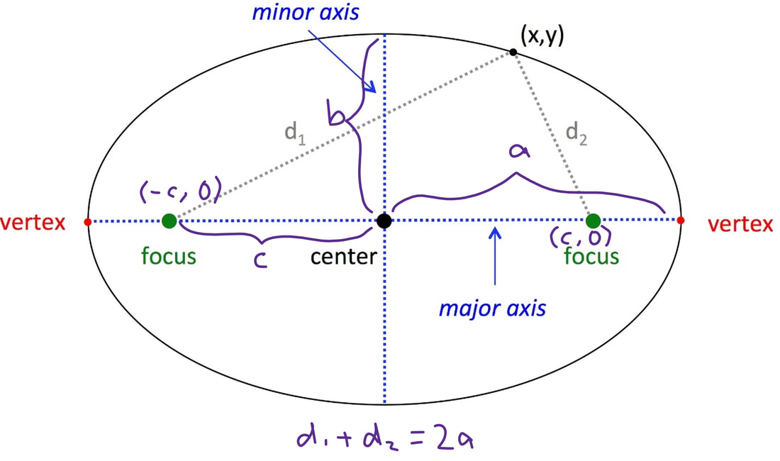 By Pythagoras’ equation, d_1 = sqrt[(x + c)^2 + y^2] and d_2 = sqrt[(c - x)^2 + y^2]. By applying this to the point (0, b) we obtain d_1 = d_2 = sqrt(c^2+ b^2). Substituting this into d_1 + d_2 = 2a gives: 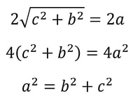 Using this information, we can use the general expressions for d_1 and d_2 to find an equation involving only x, y, a and b. 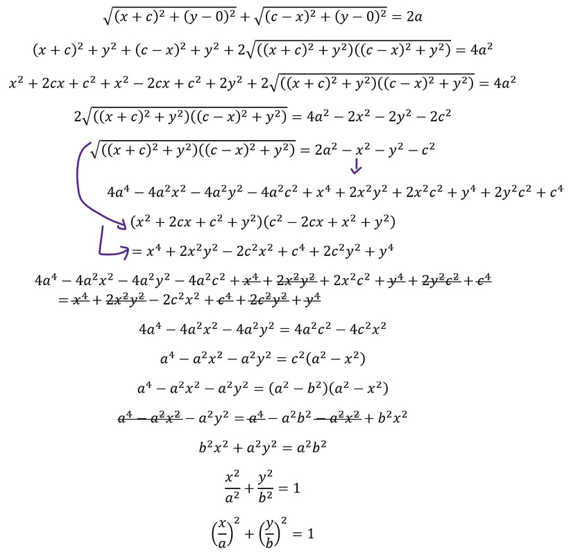 This is the standard equation for an ellipse centred at (0, 0). As with the circle and parabola equations, we can shift ellipses around by incorporating the parameters (h, k) into the equation like so: 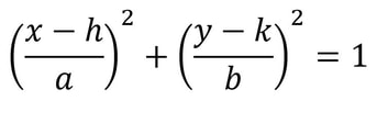 And that is the ellipse equation!
Let us know in the comments if you found these derivations useful, and what you'd like to see next!
0 Comments
Malhar Rajpal 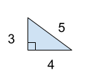 Most of us believe this fascinating finding without even questioning whether it is really true for ALL right angled triangles, and if it is, why it actually works. In this article, I will be showing you my favorite proof of the Pythagorean theorem!  Let’s say we have a square with side length a+b. We can split each side into length a and length b as shown in the diagram above. If we connect each of the splitting points (the dot in between a and b on both sides), we can see 4 right triangles which are similar since they all have sides a and b and have a right angle, as well as an additional quadrilateral area. Because the triangles are similar , we can say the third side of each of these triangles is the same length, which we can call c. This is shown in the diagram below:  To show that the quadrilateral in the centre of the diagram is a square, we need to show that it has equal side lengths (which we have already done, each side has length c), but we also need to show that it has equal angles. Since all four ABC triangles are similar and right angled, we can say that each angle enclosed by sides b and c is called θ and thus the side enclosed by the sides a and c must be equal to 180 - 90 - θ = 90 - θ, since the angles of a triangle must add up to 180 degrees. This is shown in the next diagram:  Since each side on the external square is a straight line, we can say that 90 - θ + θ + x = 180, with x being one angle of the quadrilateral surrounded by the lengths c. By solving this, we can see that x = 90 degrees, a right angle. Since there are four sides and four angles, and since all of them must be x, 90 degrees, the quadrilateral is thus proven to be a square:  So now we can compare areas. We can see the entire area of the external square is (a+b)^2 since each side of the external square is a+b. We can also represent this area as the sum of the areas of the four triangles with side lengths a, b and c and the square with side length c.
The area of the triangles is 4*(1/2)*a*b = 2ab The area of the square is c^2 So we can say (a+b)^2 = c^2 + 2ab Expanding the LHS gives a^2 + 2ab + b^2 = c^2 + 2ab, which cancels to a^2 + b^2 = c^2. This is Pythagoras' theorem! Although the theorem is named the Pythagorean Theorem after the famous Greek philosopher Pythagoras, its actual roots are actually unknown and widely debated. I have shown you one proof of the Pythagorean theorem in this article, but there are actually numerous different proofs, ranging from complex geometric proofs by extremely famed mathematicians to Einstein’s proof by dissection without rearrangement, and proofs using algebra and differentials! The uses for Pythagorean theorem are innumerable and that is why it is so famous! After all, if you are going to use it throughout your secondary education and beyond, you should know why it works! Malhar Rajpal Mathematicians pride themselves on being extremely exact and reliable with their findings. Almost always, their papers and discoveries are fully proved with no assumptions whatsoever. This contrasts most other STEM subjects, where findings are generally based on experimentation and thus have some degree of uncertainty and assumptions. You may wonder, ‘what methods of proof do mathematicians use to be absolutely confident on the validity of their findings?’. In this article, I will discuss what I think is the most beautiful and pure method of proof.
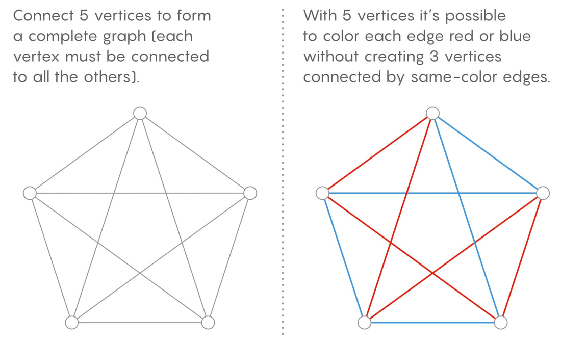
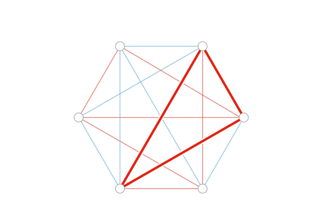
Direct proofs, or proofs by deduction, are often considered the purest form of proof since they use already proved statements or axioms to work forward and directly prove a new conjecture (a mathematical hypothesis). Let’s explore this through an example: Conjecture (statement to prove): n^3 - n is divisible by 6 for all integers n. Lemma 1 (already proven argument): if an integer is divisible by both 2 and 3, it must be divisible by 6 Thus we have to show that n^3 - n is divisible by both 2 and 3. We can begin by simply rearranging n^3 - n = n(n^2 - 1) by factoring out the n. Lemma 2: The difference of squares rule states that for some real numbers a and b, a^2 - b^2 = (a-b)(a+b). This can be shown by simple expansion of (a-b)(a+b). Thus by lemma 2, n^2 - 1 = (n-1)(n+1) and n(n^2-1) = n(n-1)(n+1). By rearranging, n(n-1)(n+1) = (n-1)n(n+1), which is the product of the three consecutive integers n-1, n, and n+1. Helper Conjecture: The product of three consecutive integers is divisible by 3. Let us prove this conjecture. In any set of three consecutive integers, one will be divisible by 3, as multiples of 3 appear every 3 consecutive integers. Since one of the three integers contributing to the product is divisible by 3, the product will have a factor of 3, and therefore be divisible by 3 itself. Helper Conjecture 2: The product of three consecutive integers is divisible by 2 Any set of two consecutive integers will have one number that is divisible by 2, by the same logic as above. Therefore, in a set of three consecutive integers, there will be at least one number that is even (divisible by 2). So their product will have at least one factor of 2, and will thus itself by divisible by 2. We have proved that n^3 - n = (n-1)(n)(n+1), which is the product of the three consecutive integers, n-1, n, and n+1. We have also shown that the product of three consecutive integers is divisible by both 2 and 3. Thus by using lemma 1 which states that any number n that is divisible by 2 and 3 is also divisible by 6, it is thus proven that the product of three consecutive integers is divisible by 6 and thus (n-1)(n)(n+1) must also be divisible by 6, for all integers n. Since n^3 - n = (n-1)(n)(n+1), and (n-1)n(n+1) is divisible by 6, our initial conjecture stating that n^3 - n is divisible by 6 for all integers n is proven. And since mathematicians like to end proofs with this sign, I will do it here too: Q.E.D. Nitya Nigam After over 70 years of effort, mathematicians have finally made headway on one of graph theory’s most confounding puzzles. In September (sorry for the article backlog, we’ve been swamped), Asaf Ferber of UC Irvine and David Conlon of Caltech, published a proof that provides the closest approximation yet for “multicolour Ramsey numbers”, which are measures of how large graphs can get before they start to contain patterns. Graphs are groups of nodes (points) and edges (lines connecting the points) - Malhar’s articles on search algorithms make extensive use of these mathematical constructs. This development gives mathematicians a deeper understanding of the relationship between order and randomness in graphs, which is of fundamental importance to the field. As described by Maria Axenovich of the Karlsruhe Institute of Technology in Germany, “there are always clusters of order [in graphs], and the Ramsey numbers quantify it.” More specifically, the Ramsey number for a given pair of parameters (number of colours and clique size) is the minimum number of vertices a perfect graph can have for which it is impossible to colour the graph without having a monochromatic clique of the specific clique size. There’s a lot of unfamiliar terminology in this definition, so let’s unpack some of the words that are probably new to you in this context: Colour: In the context of Ramsey numbers, mathematicians are interested in finding out the ways in which the edges of a graph can be coloured. Colouring is essentially just a simple way to separate edges into distinct groups. Clique: A subset of vertices in a graph such that every vertex is connected to every other member of the subset via at least one edge. Monochromatic clique: A clique where all of the edges are the same colour. Perfect graph: A perfect graph of size k is a graph with k vertices where every vertex is connected to every other vertex by exactly one edge. Now that we understand these terms, let’s take a look at an example (diagrams from Quanta Magazine):
Ramsey numbers are difficult to calculate because the complexity of a graph increases extremely quickly as vertices are added. There are simply too many ways to apply colours for these numbers to be calculated manually, and the task quickly becomes too complicated even for computers. In 1935, Paul Erdos and George Szekeres proved that the lower and bounds on 2-colour Ramsey numbers were sqrt(2)^t and 4^t respectively, where t is the clique size. Clearly, there is a huge difference between these bounds, especially as t gets large.
Using a mixture of deterministic and probabilistic methods (described both in this article and in the original paper - let us know in the comments if you’d like us to give you a more basic explanation of their methods), Ferber and Conlon improved Erdos’ lower bounds for the three- and four-colour cases from sqrt(3)^t and sqrt(4)^t = 2^t to 1.834^t and 2.135^t. While these not may seem like huge differences, these new bounds prove that exponentially larger 3- and 4-coloured graphs exist which don’t have monochromatic cliques of the specific sizes. Essentially, they established that disorder is present in larger graphs than was previously thought. Let us know in the comments if you'd like to learn more about Ramsey numbers of graph colouring! Malhar Rajpal If you ask most mathematicians what the most beautiful identity in maths is, they would likely say Euler’s identity, or more precisely: e^(iπ) + 1 = 0, where e refers to Euler’s number (~2.71828), π is the ratio of a circle’s circumference to its diameter (~3.14159) and i is the imaginary number, sqrt(-1). Since both e and π are irrational, it is easy to see why the equation is so beautiful: two irrational numbers and an imaginary number, with seemingly nothing in common, are put together in such a way that they evaluate to a simple constant: -1. In this article, I will be using the Taylor and Maclaurin series to explain why this identity is true. The Taylor series for an infinitely differentiable function is the sum of an infinite number of terms, with each of these terms being expressed with respect to the function’s derivatives (from the 0th derivative to the infinite derivative) at a point. The Taylor series is used to approximate the values of different mathematical functions and it is represented mathematically as: 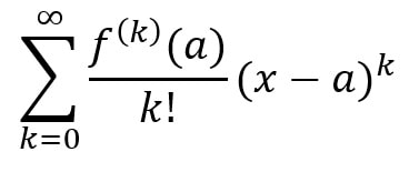 where f^(k)(a) is the k-t derivative of the function, evaluated at point a. Functions and their Taylor series are equal for most common functions. The Maclaurin series is a special case of the Taylor series centered at 0 (a=0). The Maclaurin series is therefore:  As the sum of the Maclaurin series is approximated for values of k, the function approximated by the Maclaurin series tends closer to the true function, and when k=∞, the series is equal to the real function. This video explains the concept in an intuitive way. To see why e^(iπ) + 1 = 0, let us first evaluate the Maclaurin series of cos(x) and sin(x). To figure this out, we will try to find a pattern in the derivatives of both of these functions. Let’s start with cos(x): the first derivative of cos(x) = -sin(x), the second is -cos(x), the third = sin(x), and the fourth = cos(x). Hurrah! We have found a pattern, where every multiple of four derivatives of cos(x) = cos(x) and the derivatives which follow it repeat cyclically (in the pattern cos(x) → -sin(x) → -cos(x) → sin(x) for every subsequent derivative). If we evaluate these four distinct derivatives of cos(x) at 0 we get:  And repeat. Since we have found a pattern, we can plug our values into the general Maclaurin formula. With cos(x), the Maclaurin series equals: 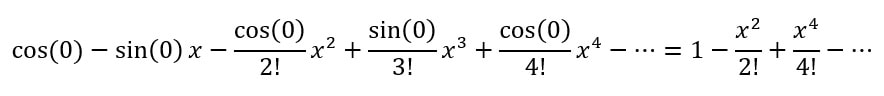 where the powers increase by two each term and are all even, and the +/- signs alternate. If this series is extended to infinite terms, it is exactly equivalent to cos(x). By following the same process with sin(x), there is a similar pattern where every k-th derivative of sin(x) is the same the (k-4)th derivative of sin(x) (when k >=4):  By following the general Maclaurin formula stated above, we can see that: 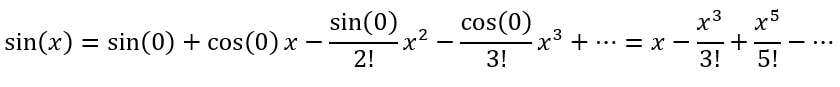 where the powers increase by two each term and are all odd, and the +/- signs alternate. We can now do the same for e^x. Since the derivative of e^x is e^x, and since e^0 = 1, we can say the Maclaurin series of e^x = e^0 + e^0 x + (e^0 x^2)/2! +(e^0 x^3)/3! + ... = 1 + x + (x^2 / 2!) + (x^3 /3!) + ... where the power increases by one each term. Now that we have shown these series, we can try and find a connection. Initially it might seem hard, however if we replace the x in ex with ix, where i is the imaginary number, we start to see a link: Since i = sqrt(-1), i^2 = -1, i^3 = -i, i^4 = 1 and i^5 = i again, we get: 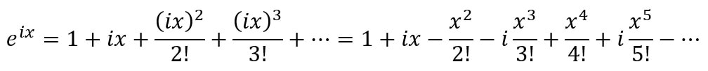 Factoring out i gives:  Do you see the connection? Yes! The first part of the expansion of e^(ix) = the Taylor expansion of cos(x) and the second part, with i factored out, = sin(x). Hence we can say that e^(ix)=cos(x) + isin(x), Euler’s formula! Neat! Now to derive Euler’s identity, all we have to do is substitute π for x in Euler’s formula to get: eiπ=cos(π) + isin(π)= -1+i*0 =-1. 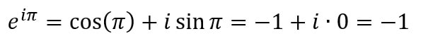 Voila: we get e^(iπ) = -1 and by adding 1 to both sides, we get Euler’s identity:
e^(iπ) + 1 = 0. Long Him Lui Sequences are a typical area of study in upper secondary mathematics. Typically, when given a sequence, we are interested in learning about the limit of a sequence. Take the following sequence (denoted x_n), as well as the following claim: 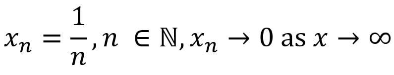 with N denoting the set of natural numbers, and the symbol ϵ meaning an element of. This can be done intuitively, which is the approach in secondary school. As n increases, the value of the reciprocal of n decreases. Since both 1 and n are positive numbers, the limit will not tend to a negative number. Therefore, the limit will lie between 0<lim x_n<1. Imagine splitting a whole pizza into more and more slices. The size of each slice of pizza will gradually decrease as the number of slices increases, so when there are infinitely many slices, the size of the slice will be extremely small; nonzero but extremely close to 0. Today, I will be discussing the rigorous definition of the limit of a sequence, and showing how it can be applied to determine the limit of a sequence. The definition is as follows: a sequence <x_n> converges to a number l (or a limit l), where l ϵ R, (R denotes the set of real numbers) if the following property holds:  The V-looking symbol denotes for all, and the backwards E denotes there exists. In words, this means that the sequence <x_n> converges to a limit l that is an element of the set of real numbers if given any ϵ > 0, so we can find a number N which is an element of the set of real numbers such that all terms of the sequence with n>N are inside a “neighborhood” (which we denote ϵ) of the value of the limit l. This definition is easier understood with the help of a diagram: 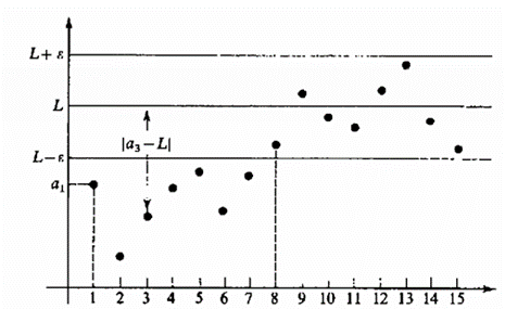 Removing the modulus, the statement |x_n - l| states that the value of |x_n - l| lies between positive and negative ϵ. Hence:  Therefore, the definition says that x_n converges to l for any specified ϵ that is small, and there is a term x_N of the sequence such that all subsequent terms lie in between l and ϵ. Looking at the diagram above, that value of N that would satisfy the given ϵ would be N=7, since all subsequent terms n>7 of the sequence all lie within the neighborhood of ϵ. For smaller neighborhoods, the value of N would be bigger so that all subsequent terms will be within that smaller neighborhood. This shows that as the distance from the limit to positive or negative ϵ decreases, there will always exist a point N such that all the subsequent points lie in the ϵ neighborhood. This implies that the sequence is tending towards that point, but will never reach it, because the value of can get infinitely small. So using our definition of the convergence of a sequence to limit l, we can solve the limit of:  We know that the sequence tends to 0, so we can substitute l=0 and x_n=1/n:  By the definition, there exists an N that is an element of Z, (Z denoting the set of integers), with N>1/ϵ: 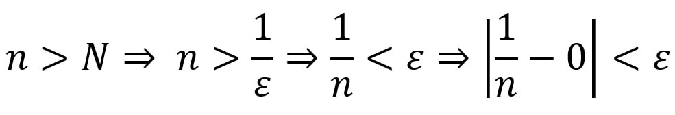 (--> denotes “implies that”) And we have returned to our original claim with the definition.
Thus, for every ϵ>0, a suitable N can be found. This specific case says that N is any integer exceeding 1/ϵ, and this concludes the proof. This definition can be applied to any sequence as long as it converges to a single specific value. If the sequence converges to positive or negative infinity, we say that the sequence diverges. Nitya Nigam Rounding numbers is a concept you were probably taught in primary school. The rule generally told to 7-year-olds is that numbers ending in 1-4 are rounded down, while numbers ending in 5-9 are rounded up (numbers ending in 0 aren’t rounded at all). This is a bit of an arbitrary rule - there are 9 numbers (1-9) that are rounded, and 5 is directly in the middle of them. It could be rounded either up or down, but convention states it should be rounded up, so we do. However, consistently rounding 5 up introduces systematic error: an error that is always wrong in a particular direction.
Let’s look at an example. Consider the numbers 0.5, 1.5, 2.5, 3.5, 4.5, 5.5, 6.5, 7.5, 8.5, and 9.5. The average of these numbers is 5. If we were to round all of these numbers as taught, you get 1, 2, 3, 4, 5, 6, 7, 8, 9 and 10. The average of these is 55/10=5.5, which is 0.5 higher than the real average. This means we have an error of 0.5 through this rounding method. A better rounding method for numbers with 5 as their last digit would be to round to the nearest even digit. This gets rid of systematic error as you would be rounding up and down equally often (at least in theory). We can see this clearer through an example. Using the same dataset as above, if we round each number to the nearest even digit, we get 0, 2, 2, 4, 4, 6, 6, 8, 8, 10. The average of this is 50/10=5, meaning we have an error of 0. Although this method of rounding 5s to the nearest even digit helps reduce error (it is actually used quite often in scientific data collection, despite it not being widely known in other contexts), it’s a bit difficult to explain to 7-year-olds. The simplification of always rounding 5 up works well enough for basic applications, but it’s important to keep in mind that it does produce a systematic error. Next time you’re taking data in a science class, try both methods of rounding, and see how much difference there is between the two! Let us know what you find in the comments section. |