|
Nitya Nigam 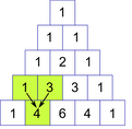 Pascal's triangle, as many of you may already know, is a mathematical pattern where the nth row is the sum of nCk from k=0 to k=n. As shown in the diagram on the left, each number is obtained by adding together the two numbers directly above it. In this article, we will investigate some of the patterns hidden in Pascal's triangle. As mentioned in the solution to May 24th's problem of the week, the sum of nCk from k=0 to k=n is 2^n, which means that the sum of rows in Pascal's triangle is 2^n. We can prove this quite easily using the binomial theorem. The binomial theorem states that:  Letting x=y=1: 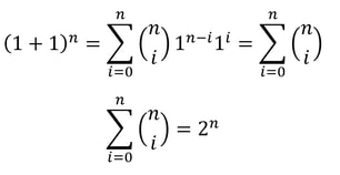 which proves our claim. Another interesting pattern in the triangle is that the squares of the numbers on the second diagonal are equal to the sum of the two numbers directly next to and below it, as shown in the diagram below: 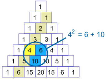 To prove this, we need to recognise that the third diagonal is the triangular numbers, which have formula n(n+1)/2. The sum of two consecutive triangular numbers is: 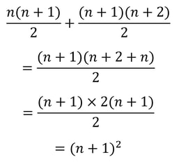 which is the necessary square number.
Pascal's triangle is full of many more interesting patterns - let us know in the comments what you'd like to learn about next!
0 Comments
Nitya Nigam As promised in March 22nd’s Problem of the Week (apologies for the delay, it’s been a busy month), this is an article explaining the connection between choose functions and polynomial functions. More specifically, we’re going to prove why sequences of the form T_n = nCk (where k is a constant integer) are equivalent to specific polynomial sequences of degree k, as well as find the specific polynomial sequence that fits our POTW. While we will be showing this algebraically, there is also a very interesting analogy to Pascal’s Triangle that shows this, which we’ll leave to our readers to think about (and share their ideas about in the comments!) The example used in our POTW was T_n = nC3 for n≥3. The first few terms of this sequence are 3C3=1,4C3=4, 5C3=10, 6C3=20. We can observe that the differences between consecutive terms (what we call the “first difference”) are 1, 3, 6, 10. While some of you may already have noticed that this sequence is the triangle number sequence, we can go a step further, observing that the difference between these differences (the second differences) are 2, 3, 4 so the third difference is constant at 1. When a sequence has its kth difference constant, the sequence can be written as a polynomial. We can prove this using basic calculus. Say we have a polynomial sequence of the following form: 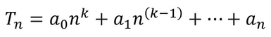 When we differentiate this, the constant term disappears, and the powers on the rest of the terms decrease by 1, giving: 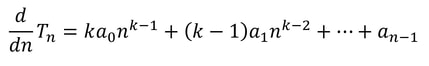 When we differentiate this k times, we get: 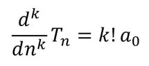 As this expression doesn’t contain any n terms, the kth derivative of a kth-degree polynomial sequence is constant. As the kth difference is simply the rate of change between integer terms, and the kth derivative is the rate of change in general (which is independent of the value of n, so will apply to integers), the two are equal. Therefore, we have shown that the kth difference of a polynomial sequence is constant, and that it is equal to k! times the coefficient on the n^k term. In our example, the third (or kth, as k=3) difference is 1. Since k! x a_0 = 1, a_0 = 1 / k! = 1 / (3x2) = 1/6. Now that we have the leading coefficient, we can simply use simultaneous equations (by plugging in the first three values of n [3, 4, 5]) to obtain the other coefficients. 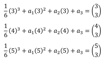 We’ll leave the process of simplifying and solving these equations to you (or your graphic calculator). The result you should get is a_1 = -1/2, a_2 = 0 and a_3 = 1/3, giving the following definition: 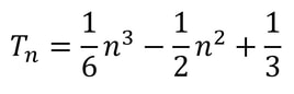 After showing this analytically for the case k=3, let’s generalise. Sequences of the form nCk can be written, from their definition, as: 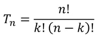 The first difference of these sequences will be T_(n+1) – T_n: 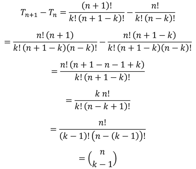 Now, if we’ve shown that the first difference of a sequence nCk is nC(k-1), then by extending this downwards by applying the same thing to the first difference sequence, we can say that the second difference is nC(k-2), and the kth difference is nC(k-k) = nC0, which is just 1. Since the kth difference is constant (which is the condition for a kth-degree polynomial sequence), these sequences can be written as polynomial sequences using the technique described above.
We hope you enjoyed this article, especially since it contained original mathematical ideas from us! Let us know in the comments if you see the link to Pascal’s Triangle, and tell us what you’d like to read next! Nitya Nigam This article is a direct result of me being hungry at the time of writing. We’ll be taking a look at the maths behind puff pastry, a deliciously light, flaky pastry made from layering dough and butter several times and then baking to crumbly perfection. It’s used in everything from dessert pies to beef wellington, and melts in your mouth. Check out this video to find out how to make it yourself. Puff pastry gets its flaky layers from a tedious rolling-and-folding process, and there are multiple techniques for this. In this article, we’ll mathematically analyse each of these techniques and discuss their advantages and disadvantages. The first rolling-and-folding technique, the Scotch method, doesn’t actually have any folding. In this method, flour, salt and cold water are combined with walnut-sized lumps of butter and mixed together. This creates flat discs of butter dispersed through the dough, rather than the continuous sheet created by other methods. Therefore, this pastry doesn’t rise as well as the others, but it is the least tedious to make. 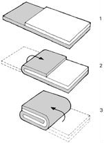 The second method is called the English method. This involves rolling the dough out into a rectangle, covering two-thirds of it in butter, and folding inwards as shown in the diagram on the left. The new rectangle is then rolled out to a thickness of about 12mm and folded again in the same way. Since each “fold” involves tripling the number of layers, the formula for the number of layers after n folds (we can call this L) is simply L = 3^n. The optimal number of layers is between 100 and 700 (depending on how much you want your pastry to rise). We can solve the following inequality to find our values of n. 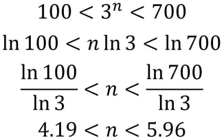 The only integer value of n between these bounds is 5, so that is the optimal number of folds. The third and final method is called the French method. Here, the dough is first rolled out into a square, and butter is placed in the middle of the square as shown in the diagram. F stands for fat (butter), and D stands for dough.  The four corners are then folded inwards, creating a smaller square. This is then rolled out into a 12mm-thick rectangle and folded as in the English method. The formula for these later folds is the same as above, but we have to use n-1 instead since the first fold is excluded. The first fold actually doubles the number of layers, since each corner is folded onto only one layer of dough. So for this method, L = 2(3^(n-1)). It is quite clear that this is less efficient than the previous method, but let’s find our optimal values of n in any case: 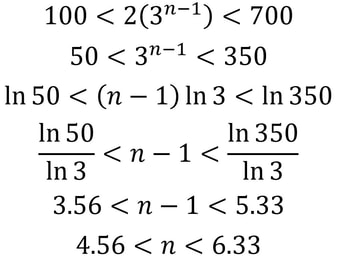 So n can be either 5 or 6 in this case.
While the English method creates more layers with less folds, it is less malleable than pastry made using the French method, since the butter was in contact with less of the dough’s surface area. Additionally, the more layers there are beyond 130, the less the pastry rises (because of the weight of all the layers), so it tends to produce a shorter pastry. Therefore it’s best used in dishes where height and texture are less important, like savoury pies where the flavour of the filling stands out. The French method is best used in delicate desserts. |