|
Malhar Rajpal In physics, a capacitor is a device that stores electrical energy. A capacitor is made up of two plates with a dielectric material between the plates. When a voltage is applied to a circuit with a capacitor, positive charge builds up on one plate while negative charge builds up on another plate, with the result being a potential difference (potential refers to the electrical potential as a result of the different charge between the plates). When the potential difference of the capacitor is the same as the voltage applied in the circuit, the current in the circuit becomes 0 and the capacitor’s p.d. stops increasing. The ‘charging’ process for the capacitor happens very quickly when there is no resistance in the circuit. If there is a resistance, by I=V/R, the current is lower and thus the charge builds up slower on the plates, slowing down the charging process. The more resistance, the slower the capacitor reaches the voltage applied. A capacitor also has a property called capacitance, C, which is the ratio of the amount of electric charge stored on a conductor to the difference in electric potential (this is directly proportional to the area of the plates and inversely proportional to the distance between the plates). The maximum charge on a capacitor is given by the equation Q = CV, where Q is charge, C is capacitance, and V is voltage. The capacitor can then be removed from the circuit with the power source and put in another circuit without a power supply. The charge then dissipates from the capacitor and flows through the circuit. This causes the absolute value of the charges on the plates and therefore the potential difference to decrease until they reach 0. The rate that the charge decreases with time of some capacitor with capacitance C depends on the resistance of the circuit and today we will explore the mathematical model finding the charge Q in this circuit at any given time while the charge dissipates. In the new loop, with the capacitor and some resistance, R, the current I of the circuit can be modelled by: I=V/R and V=IR. From above, we have the equation linking charge to capacitance and p.d.: Q = CV. Rearranging this equation, we see that V = Q/C. Substituting V = IR, IR = Q/C and thus I=Q/(RC). Current is also defined as the net rate of flow of electric charge, which can be defined mathematically as the change in charge over the change in time: ΔQ/Δt. Since charge is being dissipated (decreasing), we can say that ΔQ/Δt must be negative and, being physicists (this step is illegal is maths!), we can can say that I = -ΔQ/Δt. Now that we have two expressions for I, we can combine them: -ΔQ/Δt = Q/(RC), a differential equation! Using calculus notation, -dQ/dt=Q/(RC). Rearranging this equation, we get (1/Q)dQ = -1/(RC) dt. We can now integrate both sides: 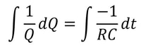 Since we don’t want the unknown constants resulting from indefinite integration in our final expression, we need to make both integrals definite (along a fixed range). We can say that we start at t=0 and go until t=t. When t=0 seconds, Q = Q_0 (initial capacitance), and when t=t seconds, we can say that Q=Q (some capacitance). So we get: 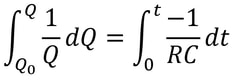 Solving this, since -1/(RC) is a constant with respect to t, we can bring it out of the integral to get: 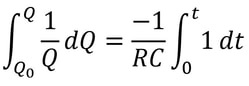 The indefinite integral of 1/Q dQ is just ln(Q) + C (natural log of Q), where C is an arbitrary constant, so by using the definite integrals, the left side of the equation is: 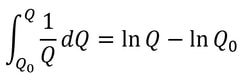 The indefinite integral of dt is just t+c and thus the right side becomes: 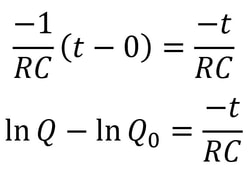 Using ln(a) - ln(b) = ln(a/b), ln(Q) - ln(Q_0) = ln(Q/Q_0). We can now raise e (Euler’s constant) to the power of both sides to get: 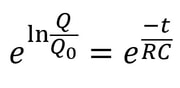 Since e^(ln(a)) = a for any a, we can rewrite as Q/Q_0= e^(-t/(RC)) and thus: 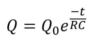 where Q is charge, Q_0 is initial charge, e is Euler’s constant, t is time since discharge begun, R is resistance, and C is capacitance.
The units of RC is seconds and it is thus be referred to as the time constant, τ. Using Q=Q_0 e^(-t/(RC)), when t = τ, Q = Q_0/e; when t = 2τ, Q = Q_0/e^2; when t = 3τ, Q = Q_0/e^3. In every discharge cycle, the time constant is equal to the amount of time taken for the charge to reduce to ~37% (1/e) of its initial value. Since charge is easily measured and this time is a constant, one great use for capacitors is in timing circuits! As an exercise for yourself, try showing that the equations V=V_0 e^(-t/(RC)) and I = (V_0 / R) e^(-t/(RC)) also hold true in RC circuits!
0 Comments
Nitya Nigam Get your power tools out and start building, because scientists from the University of Queensland in Australia have proven that time travel is theoretically possible after resolving a logical paradox. Germain Tobar and Fabio Costa used mathematical models to align classical dynamics (Newtonian physics) with general relativity (proposed by Einstein). You can find their full paper here, but we’ll be summarising its findings in the rest of this article.
You may have heard of the grandfather paradox, which is a commonly cited logical problem with the concept of time travel. If someone were to go back in time and kill their grandfather, classical dynamics states that the events following the grandfather’s demise would result in the time traveller not being born. However, relativity allows for the time traveller to use a “time loop” (formally called a closed timelike curve, or CTC) to go back in time and kill their grandfather. CTCs are essentially results of solutions to the mathematical equations of relativity. The methods used by Tobar and Costa reconcile this maths with that of classical dynamics. The two scientists used the model of the COVID-19 pandemic to work out whether the two conflicting theories could coexist. What they found is that events would realign themselves so that even if someone went back in time from t=0 and stopped COVID-19 from infecting a human at, say, t=-10000, the end result of the pandemic at t=0 would still occur. “In the coronavirus patient zero example, you might try and stop patient zero from becoming infected, but in doing so you would catch the virus and become patient zero, or someone else would,” explained Mr Tobar. Essentially, regardless of what you did as a time traveller, events would recalibrate themselves without you, meaning that the pandemic would occur and give your original self a reason to go back in time and stop it. Mr Tobar summed this up by saying: “The range of mathematical processes we discovered show that time travel with free will is logically possible in our universe without any paradox.” Dr Fabio Costa added: “The maths checks out - and the results are the stuff of science fiction.” This is truly some remarkable research, but readers must keep in mind that this paper has only been through one round of peer review, so there may be errors in the paper that haven’t been caught just yet. Furthermore, this only shows that there is a possibility for logically consistent time travel, not that this definitely can exist. But this is definitely a win for all the sci-fi nerds out there. Malhar Rajpal This is a follow-up article to one I wrote about deriving SUVAT (kinematic) equations - if you haven't read it yet, I suggest you check it out here. In this article, I will show you how to prove the last two SUVAT equations: Proof 1: s = ((v+u)/2) t This equation can be obtained by combining equations 1 and 2 (shown below) from the last article: 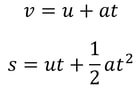 We can rearrange the first equation to find a, giving a = (v - u)/t. We can then substitute this into the second equation, which gives the following: 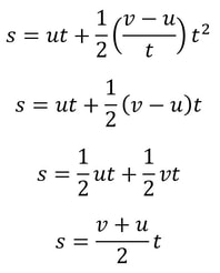 This brings us to the equation we wanted! There are also methods to derive this equation from scratch, but since we have already done the work to prove the first two equations, it makes sense to just use them. Proof 2: s = vt - 1/2 at^2 In my previous article, I proved both v = u + at and s = ut + 1/2 at^2. Rearranging v = u + at gives us u = v - at. We can now replace the u in s = ut + 1/2 at^2 with v - at to get the following: 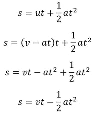 So we have proved that this equation is true as well!
I hope that you managed to figure out the proofs from the last article but if you didn’t, now you know! I find that it is always good practice to learn about how formulas are derived instead of blindly memorising them. That way, you can always be certain about what is true and what isn’t, and no one can trick you into believing a faulty formula. It is also helpful to remember what the formula is when you know where it comes from. Malhar Rajpal If you’re a high school physics student, you’ve probably encountered the 5 SUVAT equations. These are equations of motion (kinematics equations) that are used when acceleration is constant. Most students memorise and accept the equations without knowing where they came from. In this article, I will derive three of the SUVAT equations using basic calculus and explain why they work. 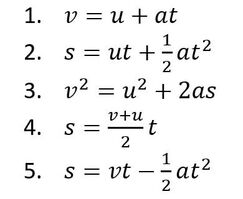 Above are the 5 SUVAT equations where s = displacement, u = initial velocity, v = final velocity, a = acceleration, t = time. Note that s, u , v, and a are all vector quantities, so they have both direction and magnitude. In this context, that means a positive quantity represents motion in one direction (e.g. upwards), and a negative quantity represents motion in the opposite direction (e.g. downwards). Proof 1: v = u + at We know acceleration is the rate of change of velocity, v, so we can say a=dv/dt. We can multiply both sides by dt to get dv = a dt. Integrating this gives the following:  When t = 0, at equals 0 and v = C. At time 0, v is the same as the initial velocity, which is u. We can therefore say that C = u, so our equation becomes v = at + u, as required. Proof 2: s = ut + (1/2)a(t^2) We know that velocity is the rate of change of displacement, s, so we can say v=ds/dt. We can multiply both sides by dt to get ds = v dt. Integrating this gives the following: 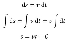 We know from equation 1 that v = u + at, so substituting this in gives: 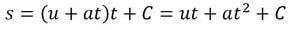 When t = 0, s = C. At time 0, displacement is also 0, since the object has not had any time to move, so C = 0. Our equation then becomes s = ut + (1/2)a(t^2), as required. Proof 3: v^2 = u^2 + 2as From the first SUVAT equation, we know that v = u + at. Squaring both sides and rearranging gives the following: 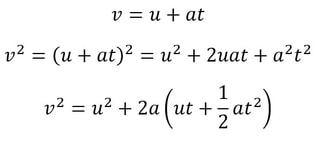 Do you see something familiar? Yes! ut + (1/2)a(t^2) the right hand side of the second SUVAT equation! By using that equation, we can replace ut + (1/2)a(t^2) with s and rewrite the initial equation as v^2 = u^2 + 2as , the third SUVAT equation!
Now that you have seen how to derive the first three SUVAT equations, I want to leave it to you to try and derive the last two SUVAT equations using either calculus or the other SUVAT equations! Don’t worry if you get stuck, because my next article will be on proving the fourth and fifth SUVAT equations! Jash Jobalia Mathematics has applications in many areas, from calculating revenue to artificial intelligence. Today, this article will talk about how mathematics can be used in the sport of table tennis. I have been playing table tennis for the past nine years, and throughout my journey I struggled with one specific shot- the lob shot (this shot is used to receive the smash shot). Therefore, I decided to use mathematics to help me decide the perfect distance from the table tennis table at which the lob shot should be hit. For these calculations there are three variables: Smash shot speed = x ms^-1 Angle at which the smash shot is hit = θ° Height at which smash shot is hit = H metres As we know the smash shot is hit at velocity x ms^-1 and angle θ°, we can find the vertical and horizontal velocity vectors of the ball by using simple trigonometric ratios, forming a right-angled triangle to do this since the table tennis table is flat. 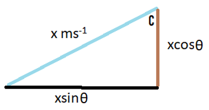 The above diagram shows the vertical and horizontal components of velocity as the smash shot is initially hit: vertical component = xcosθ and horizontal component = xsinθ. 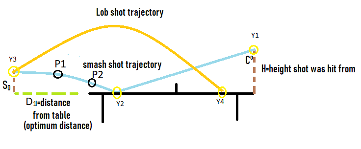 The above diagram shows the whole journey of the ball where the yellow circles represent the ball. The ball is smashed by the opponent at the point Y1, from where it travels to point Y2 where it hits the table. The ball bounces of the table and starts moving upwards till it reaches a peak at point Y3, the optimum point from where a plyer should hit the lob shot. The ball then hits the racket and moves in the trajectory shown by the orange line till it reaches point Y4, a point anywhere on the table. Now that we have understood the journey of the ball, we can start making our calculations. We need to first find the time taken by the smash shot to reach the table (from point Y1 to Y2). We will call this value of time t0 and this can be found by the kinematics equation s = ut + ½at^2, where s is vertical displacement, u is our initial vertical velocity xcosθ, and a is acceleration due to gravity 9.81 ms^-2. Since we have defined down as the positive direction (as the initial velocity is downwards), this acceleration must be positive. This gives us the following equation.  Rearranging this and applying the quadratic formula gives  where we will use the positive value of t0. We can use another kinematics equation v^2 = u^2 + 2as to find the velocity of the ball at Y2, where v is the vertical velocity at Y2, u is the vertical velocity at Y1 when the shot is hit (xcosθ), a is acceleration due to gravity and s is the displacement we found above. So, if we define the new vertical velocity component at Y2 to be V0, the following equation holds: 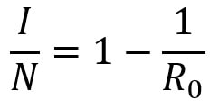 This equation lets us find V0 in terms of our initially defined variables x, θ and H, which will be useful later. At point Y2 the ball hits the table and continues moving with the same velocity after it bounces, since momentum is conserved and the mass of the ball does not change. This means the ball will move upwards after point Y2. We can define the optimum height from which the shot should be hit as S0, which is the point where the ball’s vertical velocity is 0. This makes it easier for the player to judge how to hit the shot. From here we will calculate the time (t1) it will take for the ball to reach a displacement of S0 at point Y3 where the vertical speed of the ball is zero. The vertical speed of the ball becomes zero as the ball is affected by gravity on its way up. However, to find t1 we must first find S0 by the equation v^2 = u^2 + 2as. v is 0 since the vertical velocity is 0 at point Y3; u is -V0 because it has the same magnitude as the velocity of the ball as it hits Y2 but is moving upwards so the sign is flipped; a is 9.81 ms^-2. S0 must also be negative because it is an upwards displacement. Plugging in these values gives the following: 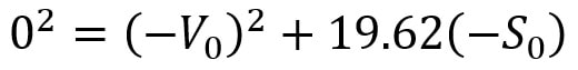
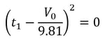
t1 can be found using s = ut + ½at^2, where u is -V0; t is t1; a is 9.81 ms^-2. 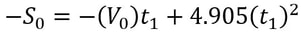 Substituting in our S0 from above and rearranging gives us the following quadratic equation: 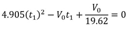
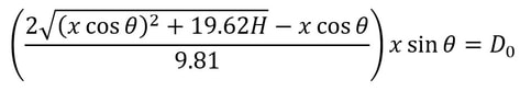
so t1 = V0 / 9.81. We know from above that (V0)^2 = (xcosθ)^2 + 19.62H, so we can substitute this into the above equation, yielding  We have now calculated t1 which we will use along with t0 to find the total horizontal distance the ball has travelled from point Y1 to Y3. Since the horizontal component of speed has remained constant throughout as we assumed there was no air resistance, we can simply use the formula distance = speed * time to calculate the horizontal distance travelled by the ball (D0) from Y1 to Y3. This can be given by the expression:  We can substitute in our expressions for t0 and t1 to obtain D0 in terms of our initial variables: 
We can now subtract the length of the table (2.74m) from D0 to give the distance in metres the player should stand from the table to hit the optimum lob shot. (D1)  This shows us some of the ways that mathematics can be used to help sports players. You can find a more detailed analysis of the maths involved in the table tennis lob shot here. For suggestions or feedback, please write to [email protected].
Nitya Nigam If you keep up with the latest developments in mathematical research, you may have heard the term “topology” being thrown around, but might not know exactly what it is. Topology is a branch of maths that studies the properties of spaces that stay the same after continuous deformation. In topology, objects can be stretched and squeezed like rubber, but they cannot be broken, so it is sometimes called “rubber-sheet geometry”. Under these rules, a triangle can be deformed into a circle, but the number 8 cannot, as it has two holes in it. So, circles and triangles are topologically equivalent, but are distinct from figure 8s. In honour of Maryam Mirzakhani’s birthday (the first woman to win a Field’s Medal, awarded to her for her groundbreaking research in topology), I thought I would write an article about one of current mathematics’ most active research fields. Links to relevant external resources are provided throughout the article in case you would like to extend your knowledge. You may wonder why topology is relevant. It has only emerged as a distinct mathematical field relatively recently; most topological research has been done after 1900. However, graph theory, which studies the properties of spaces built up from networks of vertices, edges and faces, is a form of topology. Spaces in graph theory are considered identical if all the vertices are connected up in the same way, regardless of their layout; graphs which are structurally identical but are laid out differently are called isomorphic, and are topologically equivalent. Graph theory has a wide range of applications in computer science, such as modelling computer networks, but it can also be used to optimise road networks and analyse linguistic trends. Nonetheless, the modern topological research goes far beyond graph theory, and has applications in branches of physics like vector fields and string theory. One main subfield of topology is point set topology. It analyses the local properties of spaces, and is closely related to calculus. It generalises the concept of continuity from calculus to define topological spaces, so the limits of sequences can be considered. If distances can be defined in these spaces, they are called metric spaces. In some cases, the distance cannot be defined - if a space maintains its continuity after a deformation is applied, it is still fundamentally the same space, but its “size” will have changed, so the concept of distance makes no sense. Another area of topology is algebraic topology, which instead considers the global properties of spaces. It answers topological questions by converting topological spaces into algebraic objects such as groups and rings. For example, topological spaces like the torus and the Klein bottle, pictured below, can be distinguished from each other because they have different homology groups (an algebraic concept based on integrating surfaces). Similarly, other algebraic concepts can be used to analyse and research topological spaces. 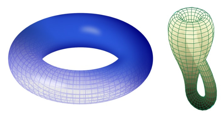 The final area of topology discussed here is differential topology, which studies spaces with some kind of smoothness associated with each point. In this field, the triangle and circle would not be equivalent to each other in terms of smoothness - the triangle has hard corners, whereas the circle has a continuously curved edge. Differential topology is particularly relevant in vector field physics, and is therefore used to study things like magnetic and electric fields. It is also helpful in describing the 4-dimensional space-time structure of our universe.
This is just an overview of the immensely complex and constantly evolving field of topology. If this article sparked your interest, you can follow the latest mathematical research explained simply at ScienceDaily. Let me know in the comments what parts of topology you find particularly intriguing, and what you’d like to read about next! |