|
Nitya Nigam If you follow tennis, you've probably seen matches where games stretch into a sixth or seventh deuce, seemingly going on forever. Theoretically, if players alternated winning points from deuce, a game could last ad infinitum - the current record is 37 deuces, set in 1975. In this article, we'll find the probability that player A wins a game of tennis from deuce, given that the probability they win a point is p. This is an obvious simplification, as the probability of a player winning a point would not stay the same throughout a match, but it makes things clear in terms of the maths. For our readers who are unfamiliar with the tennis scoring system, you can find a clear and concise guide here. Firstly, let us define some probabilities. Let P_D be the probability that player A wins given that the game is at deuce. Let P_Ba be the probability that player A wins given that player B is at AD. Let P_Aa be the probability that player A wins given that player A is at AD. Now, we can use conditional probability rules to find three equations in terms of these three probabilities and our base probability p, allowing us to solve for P_D. P_D = (prob. A wins first point)(prob. A wins from AD) + (prob. B wins first point)(prob. A wins from B at AD). The probability A wins the first point is just p, so the probability B wins the first point is 1-p. Therefore: P_D = p P_Aa + (1-p) P_Ba The conditional probability equation states that P(A|B) = P(A and B) / P(B), where P(A|B) refers to the probability of event A occurring given that event B has already occurred. In our case, P_Ba = P(A wins point | B at AD) = (p x (1-p) x P_D) / (1-p) = p P_D. Similarly, P_Aa = P(A wins point | A at AD) = (p x p x P_D) / (p) Substituting these into our equation for P_D gives: 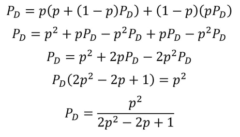 When we graph this equation, we get the following shape: 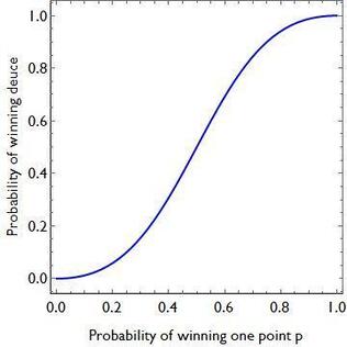 The shape of this graph is quite interesting. When p is 0.5, the probability of winning from deuce is also 0.5, so chances are even. But if p differs even slightly from 0.5, the chances of winning from deuce increase or decrease quite significantly. The shape of this graph demonstrates that players need to have very similar point probabilities for a game to be close. Given that so many matches in today's climate are very close, this shows just how close to each other the players are in ability, and how even a slight edge can have huge consequences.
Let us know in the comments if you were interested in this article about maths in sports, and tell us what you'd like to read about next!
0 Comments
Jash Jobalia Mathematics has applications in many areas, from calculating revenue to artificial intelligence. Today, this article will talk about how mathematics can be used in the sport of table tennis. I have been playing table tennis for the past nine years, and throughout my journey I struggled with one specific shot- the lob shot (this shot is used to receive the smash shot). Therefore, I decided to use mathematics to help me decide the perfect distance from the table tennis table at which the lob shot should be hit. For these calculations there are three variables: Smash shot speed = x ms^-1 Angle at which the smash shot is hit = θ° Height at which smash shot is hit = H metres As we know the smash shot is hit at velocity x ms^-1 and angle θ°, we can find the vertical and horizontal velocity vectors of the ball by using simple trigonometric ratios, forming a right-angled triangle to do this since the table tennis table is flat. 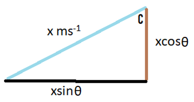 The above diagram shows the vertical and horizontal components of velocity as the smash shot is initially hit: vertical component = xcosθ and horizontal component = xsinθ. 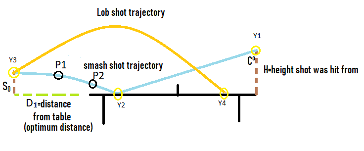 The above diagram shows the whole journey of the ball where the yellow circles represent the ball. The ball is smashed by the opponent at the point Y1, from where it travels to point Y2 where it hits the table. The ball bounces of the table and starts moving upwards till it reaches a peak at point Y3, the optimum point from where a plyer should hit the lob shot. The ball then hits the racket and moves in the trajectory shown by the orange line till it reaches point Y4, a point anywhere on the table. Now that we have understood the journey of the ball, we can start making our calculations. We need to first find the time taken by the smash shot to reach the table (from point Y1 to Y2). We will call this value of time t0 and this can be found by the kinematics equation s = ut + ½at^2, where s is vertical displacement, u is our initial vertical velocity xcosθ, and a is acceleration due to gravity 9.81 ms^-2. Since we have defined down as the positive direction (as the initial velocity is downwards), this acceleration must be positive. This gives us the following equation.  Rearranging this and applying the quadratic formula gives 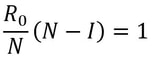 where we will use the positive value of t0. We can use another kinematics equation v^2 = u^2 + 2as to find the velocity of the ball at Y2, where v is the vertical velocity at Y2, u is the vertical velocity at Y1 when the shot is hit (xcosθ), a is acceleration due to gravity and s is the displacement we found above. So, if we define the new vertical velocity component at Y2 to be V0, the following equation holds: 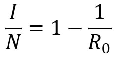 This equation lets us find V0 in terms of our initially defined variables x, θ and H, which will be useful later. At point Y2 the ball hits the table and continues moving with the same velocity after it bounces, since momentum is conserved and the mass of the ball does not change. This means the ball will move upwards after point Y2. We can define the optimum height from which the shot should be hit as S0, which is the point where the ball’s vertical velocity is 0. This makes it easier for the player to judge how to hit the shot. From here we will calculate the time (t1) it will take for the ball to reach a displacement of S0 at point Y3 where the vertical speed of the ball is zero. The vertical speed of the ball becomes zero as the ball is affected by gravity on its way up. However, to find t1 we must first find S0 by the equation v^2 = u^2 + 2as. v is 0 since the vertical velocity is 0 at point Y3; u is -V0 because it has the same magnitude as the velocity of the ball as it hits Y2 but is moving upwards so the sign is flipped; a is 9.81 ms^-2. S0 must also be negative because it is an upwards displacement. Plugging in these values gives the following: 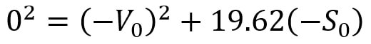
t1 can be found using s = ut + ½at^2, where u is -V0; t is t1; a is 9.81 ms^-2. 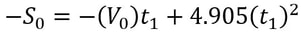 Substituting in our S0 from above and rearranging gives us the following quadratic equation: 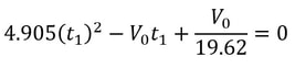
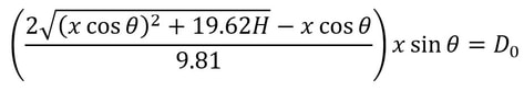
so t1 = V0 / 9.81. We know from above that (V0)^2 = (xcosθ)^2 + 19.62H, so we can substitute this into the above equation, yielding 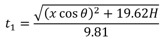 We have now calculated t1 which we will use along with t0 to find the total horizontal distance the ball has travelled from point Y1 to Y3. Since the horizontal component of speed has remained constant throughout as we assumed there was no air resistance, we can simply use the formula distance = speed * time to calculate the horizontal distance travelled by the ball (D0) from Y1 to Y3. This can be given by the expression:  We can substitute in our expressions for t0 and t1 to obtain D0 in terms of our initial variables: 
We can now subtract the length of the table (2.74m) from D0 to give the distance in metres the player should stand from the table to hit the optimum lob shot. (D1)  This shows us some of the ways that mathematics can be used to help sports players. You can find a more detailed analysis of the maths involved in the table tennis lob shot here. For suggestions or feedback, please write to [email protected].
Paul Jackson (guest writer) It might seem a little strange for me to be writing in a magazine that is ‘for students by students’. After all, I have just retired from teaching after being a Maths teacher for 43 years.
But remember the IB mission statement! The IB programmes encourage students to become lifelong learners. So I’m still a student and I wanted to share with you some of the Mathematics I’ve recently been learning. I have always enjoyed watching live sport, especially football. But recently, I have been to Rugby Union, Rugby League and Aussie Rules Football games. In all of them I became interested in the Mathematics behind the scoring systems. The first Rugby Union game I saw was a ladies’ international match, Wales v Italy in Cardiff. The final score was 22 – 15 to Italy. It got me thinking in 2 ways:
I have to say I prefer watching football, rugby is very ‘stop-go’. Too many breaks for me, I prefer the more continuous flow of a good football match. It was during the ‘stop’ periods that I spent my time thinking mathematically, though! If you try problems 1 and 2 above, do submit your answers to Integral Magazine (via email) who will publish the best one. If you are interested in any of these sports, or any other sport with an interesting scoring system, do some mathematics and submit your answers to Integral Magazine. I would be interested to see what you find. If you would like to read more on this, see my article on my website. Nitya Nigam In today’s article, I’d like to take a look at what a problem that arose in my maths class this week. What seems to be a simple matter of arranging teams quickly turns into a complicated counting problem involving several stages of thinking. First, I’d like to introduce two concepts that most of our readers are probably familiar with, but are crucial to understanding counting problems, so I will go over them for the benefit of those who may not have heard of them. Permutations are ways to arrange things which take into account the order they are in. For example, there are 6 ways to arrange the letters ABC: ABC, ACB, BAC, BCA, CAB and CBA. We can quantify the ways to permute n objects as n! which means in the above case we should have 3! = 6 ways to arrange the 3 letters, which checks out. Combinations are ways to arrange things when the order does not matter. If we wanted to choose 3 distinct ice cream flavours from 8 different possible flavours, we could do this in 8x7x6 ways, but we would then have to divide by 3! = 6 to account for the fact we overcounted by including different orderings (if we did not divide by 3!, we would have counted chocolate, vanilla, strawberry and vanilla, chocolate, strawberry as different choices, even though we do not care about ordering in this case). We now have the tools to tackle the problem from my maths class. Consider the problem of arranging 8 different football teams into 4 different quarter-finals. How many different ways can this be done? At first, this may seem like a simple question. If we consider the first quarter-final, there are (8x7)/2 = 28 ways to choose 2 teams from the 8. There are (6x5)/2 = 15 ways to choose 2 teams from the remaining 6, (4x3)/2 = 6 ways to choose 2 teams from the remaining 4, and (2x1)/2 = 1 ways to choose 2 teams from the last 2 (obviously). So, there are 28x15x6x1 = 2520 ways to arrange 8 teams into quarter-finals. However, this is not the only way to approach the problem. There are 8! = 40320 ways to arrange 8 teams in a list. For the purposes of this problem, it does not matter whether a pair of teams A and B are in positions 1 and 2, or if positions 1 and 2 are held by B and A respectively, because they would be playing each other regardless. This applies to the teams in positions 3 and 4, 5 and 6 as well as 7 and 8. This means there are 24 instances of overcounting, so we divide 40320 by 24 = 16 to get 2520, which is the same answer we arrived at above. Although it is satisfying to be able to arrive at the same answer through two different methods, the number we obtained is not strictly correct in terms of meaningfully different games. Consider the diagram below, which shows one half of the quarter-finals.  Regardless of whether AB and CD are arranged AB, CD or CD, AB (with rearranging possible within the two pairs as well), the semi-final matchup will be the same - one team from the AB pair, and one team from the CD pair. This means our method above is overcounting, so now we need to figure out by how much we are overcounting so that we can account for the discrepancy.
Essentially, our first method failed to account for the fact that the draw A-B, C-D, E-F, G-H is indistinguishable from the draw A-B, G-H, C-D, E-F. There are 4! = 24 different ways to rearrange the 4 quarter-final pairings, so dividing 2520 from above by 24 gives us our final answer of 105 meaningfully different draws. Once again, we can arrive at this same answer through a different route. It is easier to first consider the simpler case of just 4 teams (semi-finals). If the 4 teams are A, B, C and D, you can pair A with either B, C or D (3 choices) and there is only one choice for the remaining pair, so there are 3 ways to arrange 4 teams. If there are 6 teams, you have 5 choices for who to pair A with, and then 3 choices to arrange the remaining 4 teams (as calculated in the isolated 4 team case), so there are a total of 5x3 = 15 ways to arrange the 6 teams. Moving on the 8 team case, the number of arrangements is then simply 7 times the number of arrangements for 6 teams, so our answer is 7x15 = 105. The objective of this article was to show how complex even deceptively simple problems can be, not to dissuade our readers, but to encourage careful critical thinking from the start of tackling a problem. We have also demonstrated how problems can be solved using multiple different, but equally valid, methods. Let us know in the comments what you would like to read about next! |