|
Malhar Rajpal This is a follow-up article to one I wrote about deriving SUVAT (kinematic) equations - if you haven't read it yet, I suggest you check it out here. In this article, I will show you how to prove the last two SUVAT equations: Proof 1: s = ((v+u)/2) t This equation can be obtained by combining equations 1 and 2 (shown below) from the last article: 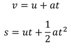 We can rearrange the first equation to find a, giving a = (v - u)/t. We can then substitute this into the second equation, which gives the following: 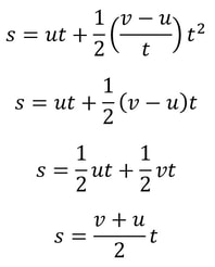 This brings us to the equation we wanted! There are also methods to derive this equation from scratch, but since we have already done the work to prove the first two equations, it makes sense to just use them. Proof 2: s = vt - 1/2 at^2 In my previous article, I proved both v = u + at and s = ut + 1/2 at^2. Rearranging v = u + at gives us u = v - at. We can now replace the u in s = ut + 1/2 at^2 with v - at to get the following: 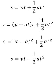 So we have proved that this equation is true as well!
I hope that you managed to figure out the proofs from the last article but if you didn’t, now you know! I find that it is always good practice to learn about how formulas are derived instead of blindly memorising them. That way, you can always be certain about what is true and what isn’t, and no one can trick you into believing a faulty formula. It is also helpful to remember what the formula is when you know where it comes from.
6 Comments
Nitya Nigam This article is a direct result of me being hungry at the time of writing. We’ll be taking a look at the maths behind puff pastry, a deliciously light, flaky pastry made from layering dough and butter several times and then baking to crumbly perfection. It’s used in everything from dessert pies to beef wellington, and melts in your mouth. Check out this video to find out how to make it yourself. Puff pastry gets its flaky layers from a tedious rolling-and-folding process, and there are multiple techniques for this. In this article, we’ll mathematically analyse each of these techniques and discuss their advantages and disadvantages. The first rolling-and-folding technique, the Scotch method, doesn’t actually have any folding. In this method, flour, salt and cold water are combined with walnut-sized lumps of butter and mixed together. This creates flat discs of butter dispersed through the dough, rather than the continuous sheet created by other methods. Therefore, this pastry doesn’t rise as well as the others, but it is the least tedious to make.  The second method is called the English method. This involves rolling the dough out into a rectangle, covering two-thirds of it in butter, and folding inwards as shown in the diagram on the left. The new rectangle is then rolled out to a thickness of about 12mm and folded again in the same way. Since each “fold” involves tripling the number of layers, the formula for the number of layers after n folds (we can call this L) is simply L = 3^n. The optimal number of layers is between 100 and 700 (depending on how much you want your pastry to rise). We can solve the following inequality to find our values of n. 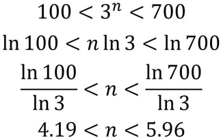 The only integer value of n between these bounds is 5, so that is the optimal number of folds. The third and final method is called the French method. Here, the dough is first rolled out into a square, and butter is placed in the middle of the square as shown in the diagram. F stands for fat (butter), and D stands for dough. 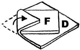 The four corners are then folded inwards, creating a smaller square. This is then rolled out into a 12mm-thick rectangle and folded as in the English method. The formula for these later folds is the same as above, but we have to use n-1 instead since the first fold is excluded. The first fold actually doubles the number of layers, since each corner is folded onto only one layer of dough. So for this method, L = 2(3^(n-1)). It is quite clear that this is less efficient than the previous method, but let’s find our optimal values of n in any case: 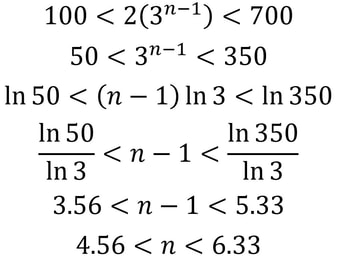 So n can be either 5 or 6 in this case.
While the English method creates more layers with less folds, it is less malleable than pastry made using the French method, since the butter was in contact with less of the dough’s surface area. Additionally, the more layers there are beyond 130, the less the pastry rises (because of the weight of all the layers), so it tends to produce a shorter pastry. Therefore it’s best used in dishes where height and texture are less important, like savoury pies where the flavour of the filling stands out. The French method is best used in delicate desserts. Malhar Rajpal If you’re a high school physics student, you’ve probably encountered the 5 SUVAT equations. These are equations of motion (kinematics equations) that are used when acceleration is constant. Most students memorise and accept the equations without knowing where they came from. In this article, I will derive three of the SUVAT equations using basic calculus and explain why they work. 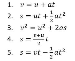 Above are the 5 SUVAT equations where s = displacement, u = initial velocity, v = final velocity, a = acceleration, t = time. Note that s, u , v, and a are all vector quantities, so they have both direction and magnitude. In this context, that means a positive quantity represents motion in one direction (e.g. upwards), and a negative quantity represents motion in the opposite direction (e.g. downwards). Proof 1: v = u + at We know acceleration is the rate of change of velocity, v, so we can say a=dv/dt. We can multiply both sides by dt to get dv = a dt. Integrating this gives the following: 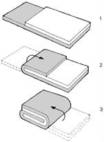 When t = 0, at equals 0 and v = C. At time 0, v is the same as the initial velocity, which is u. We can therefore say that C = u, so our equation becomes v = at + u, as required. Proof 2: s = ut + (1/2)a(t^2) We know that velocity is the rate of change of displacement, s, so we can say v=ds/dt. We can multiply both sides by dt to get ds = v dt. Integrating this gives the following: 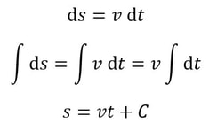 We know from equation 1 that v = u + at, so substituting this in gives: 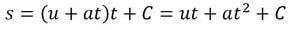 When t = 0, s = C. At time 0, displacement is also 0, since the object has not had any time to move, so C = 0. Our equation then becomes s = ut + (1/2)a(t^2), as required. Proof 3: v^2 = u^2 + 2as From the first SUVAT equation, we know that v = u + at. Squaring both sides and rearranging gives the following: 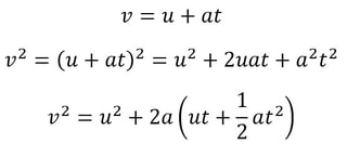 Do you see something familiar? Yes! ut + (1/2)a(t^2) the right hand side of the second SUVAT equation! By using that equation, we can replace ut + (1/2)a(t^2) with s and rewrite the initial equation as v^2 = u^2 + 2as , the third SUVAT equation!
Now that you have seen how to derive the first three SUVAT equations, I want to leave it to you to try and derive the last two SUVAT equations using either calculus or the other SUVAT equations! Don’t worry if you get stuck, because my next article will be on proving the fourth and fifth SUVAT equations! Nitya Nigam A few weeks ago, we wrote about end-to-end encryption and examined the maths behind the Diffie-Hellman key exchange. Continuing on the theme of cryptography, today’s article will talk about pseudorandomness, an important concept to many fields, including complexity theory, combinatorics, number theory, and, of course, cryptography. This article hopes to leave you with a fundamental understanding of why pseudorandomness is so important, and the structures that underpin its study.
Firstly, what is pseudorandomness? As you can probably guess from its word root, it essentially means “fake randomness”. True randomness, as is seen in radioactive decay and quantum phenomena, cannot be truly replicated by computers, which are deterministic - they run on Boolean logic (let us know in the comments if you’d like to read an article about this), not probability. But being able to replicate randomness is an important tool for mathematicians and computer scientists alike. It has applications as simple as generating winning lottery numbers and as complex as simulating nuclear fission. In these situations and more, it is important to have a way to generate numbers in an unpredictable pattern. As we discussed in our article on encryption, messages can be made secret using keys. Cryptosystems are most secure when these keys are random, so that they cannot easily be guessed by an interceptor, which is why randomness is so important in the field. Pseudorandom number generators rely on a special type of mathematical concept called one-way functions. These are functions that are easy to perform in one direction, but are near-impossible to reverse. The process of modular exponentiation discussed in our encryption article is an example of a one-way function, but the most commonly cited example of such functions is multiplying two large prime numbers together. This is an easy process, but factoring the large product back into its prime components is very computationally inefficient. There are three steps that link pseudorandom number generators to one-way functions. First, let’s define our generator, G, as unpredictable if every polynomial-time algorithm struggles to predict the nth number from the first n-1 numbers. Note that this definition only covers numbers already generated, and doesn’t extend to how generators actually generate new numbers. That is where one-way functions come in. For G to be pseudorandom, it must first be unpredictable. However, if G is not pseudorandom, then G is predictable. If G is not pseudorandom, then there must be some algorithm that can distinguish between outputs of G and a uniformly sampled string with non-negligible accuracy, and a bit of maths too complicated for us to cover called Yao’s Theorem states that the latter cannot be the case, so all unpredictable generators are also pseudorandom. To turn G into a proper generator, we need to show that it is possible for G to generate new numbers that cannot be predicted to a non-negligible degree of accuracy. The Goldreich-Levin Theorem (the proof of which is also too complex to go into here) states that one-way functions can be used to stretch the output of a generator by one number, allowing for pseudorandomness to be achieved. Our generator G needs a number called a pseudorandom seed to get started, as one-way functions can only extend strings, not create them. If this seed is kept secret, though, such generators serve as effective ways of generating random keys for encrypted communication. Understanding pseudorandomness also has more tangible benefits. In 2003, Mohan Srivastava, a statistician in Canada, discovered that the Ontario Lottery was using a pseudorandom number generator for its scratch cards, so cards with a row containing three numbers that each appear only once within the card’s visible numbers were almost always winners. This is because pseudorandomness follows a specific probability distribution, based on the one-way function it uses. Instead of gaming the system and keeping the money for himself, Srivastava sent the Ontario Lottery and Gaming Corporation 20 unscratched cards, each marked as either winners or losers. Two hours later, he got a call telling him he had correctly identified 19 out of the 20 cards. The game was discontinued the next day. I hope this article has left you with a better understanding of pseudorandomness and its uses. Let us know in the comments if you have any questions, and tell us what you’d like to read about next! Nitya Nigam Although there are many things we don’t know about COVID-19, there is one thing we do know: the pandemic will only end once enough people are immune to the virus, causing its spread to slow and eventually stop. At this point, whether immunity is obtained through people being infected or vaccinated, the population will have developed “herd immunity”. This threshold is an important figure to consider, since it informs decisions about how many vaccines need to be produced and when places can lift lockdowns and reopen. However, calculating this threshold is a complex process. To understand how we get to the herd immunity threshold, we need to derive an equation. If you’ve been reading about COVID-19, or know about the spread of disease, you should be familiar with the term R0, which refers to the average number of people infected by one infected person. R0 acts as a measure of how quickly a disease can spread. If R0 is 1, then the spread of infection follows a linear track - each infected person infects one more, who can only infect one other person, and so on. However, if R0 is larger than 1, the spread quickly becomes exponential. If R0 is 2, then the first patient can infect two other people, who can each infect two more causing 4 infections, then 8, then 16 and so forth. Therefore, our goal with herd immunity is to bring the number of people infected by a single patient down to 1, or even less. Say you are infected with COVID-19, and have a population of 10 people that you interact with. If we set R0 to be 2, then two of the 10 people get infected. This means that the chance of somebody getting infected is 20%. However, if five of your friends are vaccinated or have already had COVID-19, they would be immune to the disease. This means that there are only five remaining friends who could fall sick. The same probability of 20% applies to them, so only 0.2*5 = 1 of them will be infected. We can generalise this process for any value of R0. If we assume that each infected person comes into contact with N people in each time period (usually a day), then we can expect R0/N people to be infected on average. If there are immune people in the population (we can call this number I), then the number of new infections can be represented by the following expression:  We want this to equal 1, so we have the equation: 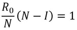 We want to solve this for I/N, which represents the proportion of the population that needs to be immune. Rearranging for this gives 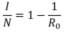 So our formula for the herd immunity threshold is just 1-(1/R0). 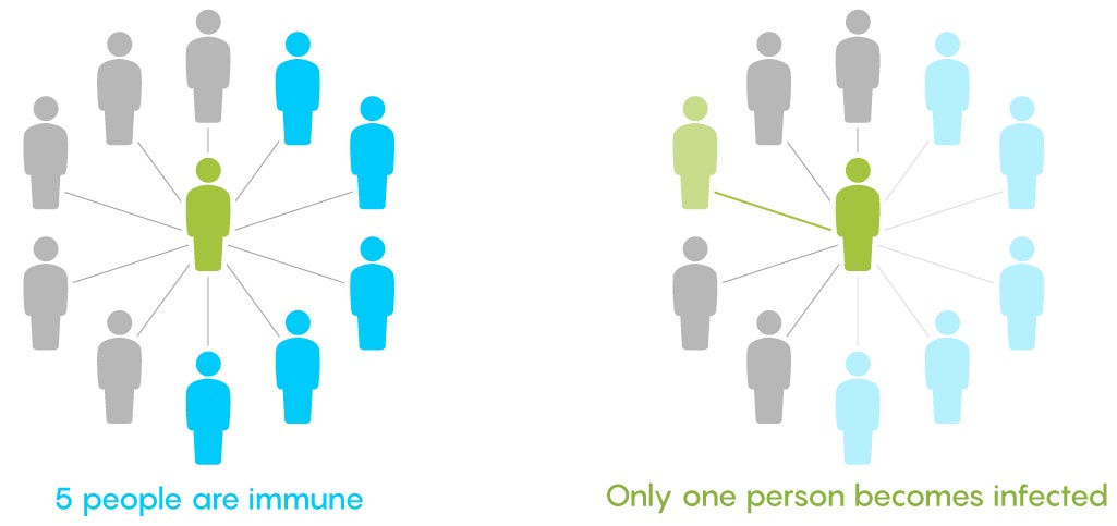 However, finding an R0 value is more difficult than it may seem. R0 values can vary hugely by location - urban areas can have R0 values more than twice as high as country averages. There are also biological differences between people that can make them more likely to get infected. These biological variations, which are results of both genetic makeup and environmental factors, are referred to by epidemiologists as the “heterogeneity of susceptibility”. For example, R0 values would be much higher in places like nursing homes, where elderly people are far likelier to fall ill. On a broad scale though, heterogeneity tends to lower the herd immunity threshold. At first, the virus will spread to people who are more susceptible, but once most of these susceptible individuals are infected, the spread of the virus will slow.
There is disagreement in the scientific community regarding what the herd immunity threshold for COVID-19 really is. Standard models indicate that 60% of the US population would need to be vaccinated for herd immunity to be achieved, but some experts place the value between 40% and 50%. Another (non-peer-reviewed) study done in May suggests that the value could be as low as 20%. While the scientists debate, however, the best thing to do is prevent the spread of the virus and decrease the R0 value as far as possible. Social distancing, mask-wearing and widespread testing are our best bets to keep people safe and healthy until vaccines are widely available. Malhar Rajpal Imagine you have a complex maze with hundreds of ways to reach the endpoint. How do you find the shortest route? This is the exact problem that appears in a vast array of real-world problems from GPS navigation to tracing garbage collection. You could split the problem into an unweighted graph, where each position in the maze or street on the map is a node, and try to manually trace the different solutions from the initial position (also known as the root node) to the solution. But you will soon find that, since there are so many different routes, solving this problem manually is a near-impossible task! You need to use a computer algorithm, and luckily for you, the solution comes in the form of Breadth First Search (BFS), which explores each node in the unweighted graph until the solution is reached. To explain the concept of BFS, I will use a basic example: 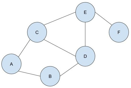 L circle (node) A be our root node, and we must traverse our way to node F, which is our end node, or solution. We could analogise each of the nodes in the graph to be a certain street, and each of the lines show which streets are connected (for example street A is directly connected to street B or street C). There are obviously several ways to get from node A to node F (two of which could be A → B → D → E → F or A → C → D → E → F), but we want to get to node F by traversing through the least amount of nodes or streets. How would the algorithm do this? The answer is not as complex as you may think. The algorithm requires a list (more formally called a frontier). This frontier contains the nodes that are currently being explored. Another list is also needed which contains the explored nodes. When the algorithm initialises, node A (our first node) is put into our frontier (as shown below) since it is the first to be explored. The list containing the explored nodes remains empty. 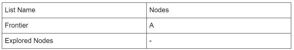 The frontier makes use of a queue data structure which, simply put, will always explore the first node that was appended in a list (in this case our frontier). Since node A is our only node, and hence the first node, it is explored. The exploration process includes checking if the current node is equal to the solution node. If it is, then the program can return the path needed to reach the final node. If not, the program will check if any of the directly connected nodes to the current node is in the ‘Explored Nodes’ list. The program will then simply add all the connected nodes that are not in the ‘Explored Nodes’ list to the frontier. So in our example, since node B and C are directed connected to A, and since neither node B or C are in the explored nodes list, they are both added to the frontier like so: 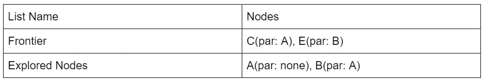 Since node A is now explored and a queue is a first in first out data structure, meaning the first node in the list is the node that is removed when needed (when a node is removed from a queue, it can only be the first first node in the list). Node A is then added to the explored nodes: 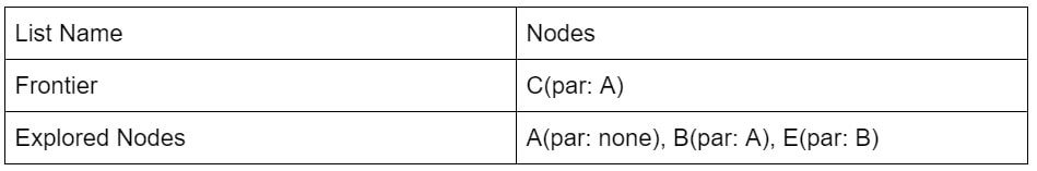 Each node contains the needed data (street name etc.) as well as the parent node within itself. For example, node B contains its own information as well as its parent element (node A). These parents will be labelled in our table using the format ‘par: letter of node’. Now, since node B is the first node in our frontier, it follows the same process as before: it is checked whether it is the solution node (node F). Since it’s not, the program gets all its connected nodes: node A and node D. Since node A is already explored, it is ignored (this avoids backtracking) and node D (with its parent being node B) is added to the frontier. Node B is then added to the explored nodes. 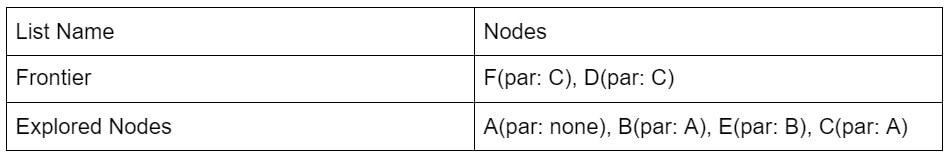 This process is continued until we arrive at the following table: 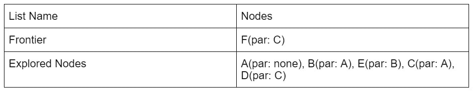 Finally node F is our solution. Since we kept track of the parents, we can easily backtrack the optimal route from the solution node (Node F) all the way to the initial node. We can do this by creating a list and adding the subsequent parent elements of each of the previous nodes to the list, until we reach node A (which has par:none). This gives us this list: (F, E, C, A). Reversing this list, we can find the shortest route to node F: Node A → Node C → Node E → Node F (shown in red on the below diagram), which only traverses through four nodes! This is great since our programs can easily perform each exploration in a matter of milliseconds, allowing incredibly complex search problems to be entirely solved in as little as a couple of seconds! 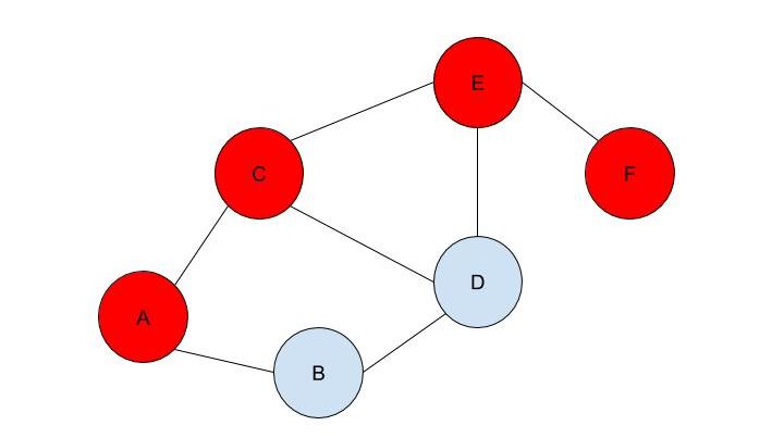 BFS is a widely used algorithm, effective in finding the shortest route from one node to another. Although complex problems like GPS navigation systems use slightly different algorithms since they must take into account several different aspects (traffic, speed limits etc.), these algorithms are all built upon the fundamental principles of BFS. If you want to go deeper into the world of search algorithms, I would suggest looking at A* search, which finds the route between two nodes with the lowest cost (cost referring to some variable; it could be lowest time, lowest distance etc.).
Jash Jobalia Mathematics has applications in many areas, from calculating revenue to artificial intelligence. Today, this article will talk about how mathematics can be used in the sport of table tennis. I have been playing table tennis for the past nine years, and throughout my journey I struggled with one specific shot- the lob shot (this shot is used to receive the smash shot). Therefore, I decided to use mathematics to help me decide the perfect distance from the table tennis table at which the lob shot should be hit. For these calculations there are three variables: Smash shot speed = x ms^-1 Angle at which the smash shot is hit = θ° Height at which smash shot is hit = H metres As we know the smash shot is hit at velocity x ms^-1 and angle θ°, we can find the vertical and horizontal velocity vectors of the ball by using simple trigonometric ratios, forming a right-angled triangle to do this since the table tennis table is flat. 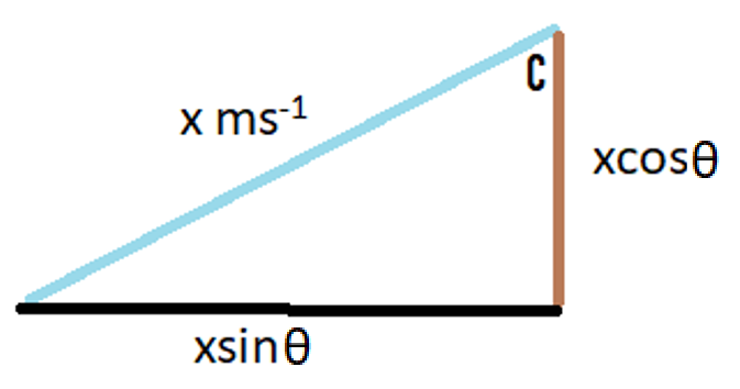 The above diagram shows the vertical and horizontal components of velocity as the smash shot is initially hit: vertical component = xcosθ and horizontal component = xsinθ. 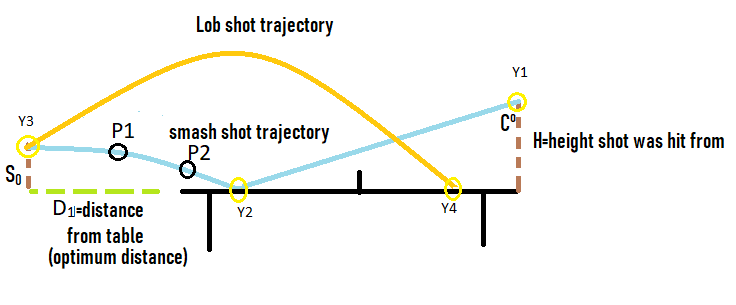 The above diagram shows the whole journey of the ball where the yellow circles represent the ball. The ball is smashed by the opponent at the point Y1, from where it travels to point Y2 where it hits the table. The ball bounces of the table and starts moving upwards till it reaches a peak at point Y3, the optimum point from where a plyer should hit the lob shot. The ball then hits the racket and moves in the trajectory shown by the orange line till it reaches point Y4, a point anywhere on the table. Now that we have understood the journey of the ball, we can start making our calculations. We need to first find the time taken by the smash shot to reach the table (from point Y1 to Y2). We will call this value of time t0 and this can be found by the kinematics equation s = ut + ½at^2, where s is vertical displacement, u is our initial vertical velocity xcosθ, and a is acceleration due to gravity 9.81 ms^-2. Since we have defined down as the positive direction (as the initial velocity is downwards), this acceleration must be positive. This gives us the following equation.  Rearranging this and applying the quadratic formula gives  where we will use the positive value of t0. We can use another kinematics equation v^2 = u^2 + 2as to find the velocity of the ball at Y2, where v is the vertical velocity at Y2, u is the vertical velocity at Y1 when the shot is hit (xcosθ), a is acceleration due to gravity and s is the displacement we found above. So, if we define the new vertical velocity component at Y2 to be V0, the following equation holds: 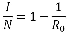 This equation lets us find V0 in terms of our initially defined variables x, θ and H, which will be useful later. At point Y2 the ball hits the table and continues moving with the same velocity after it bounces, since momentum is conserved and the mass of the ball does not change. This means the ball will move upwards after point Y2. We can define the optimum height from which the shot should be hit as S0, which is the point where the ball’s vertical velocity is 0. This makes it easier for the player to judge how to hit the shot. From here we will calculate the time (t1) it will take for the ball to reach a displacement of S0 at point Y3 where the vertical speed of the ball is zero. The vertical speed of the ball becomes zero as the ball is affected by gravity on its way up. However, to find t1 we must first find S0 by the equation v^2 = u^2 + 2as. v is 0 since the vertical velocity is 0 at point Y3; u is -V0 because it has the same magnitude as the velocity of the ball as it hits Y2 but is moving upwards so the sign is flipped; a is 9.81 ms^-2. S0 must also be negative because it is an upwards displacement. Plugging in these values gives the following: 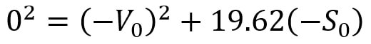
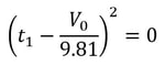
t1 can be found using s = ut + ½at^2, where u is -V0; t is t1; a is 9.81 ms^-2. 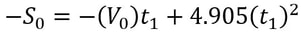 Substituting in our S0 from above and rearranging gives us the following quadratic equation: 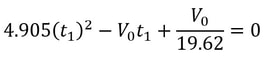
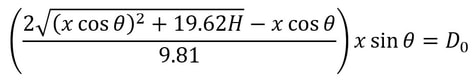
so t1 = V0 / 9.81. We know from above that (V0)^2 = (xcosθ)^2 + 19.62H, so we can substitute this into the above equation, yielding 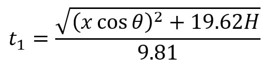 We have now calculated t1 which we will use along with t0 to find the total horizontal distance the ball has travelled from point Y1 to Y3. Since the horizontal component of speed has remained constant throughout as we assumed there was no air resistance, we can simply use the formula distance = speed * time to calculate the horizontal distance travelled by the ball (D0) from Y1 to Y3. This can be given by the expression: 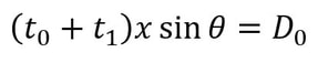 We can substitute in our expressions for t0 and t1 to obtain D0 in terms of our initial variables: 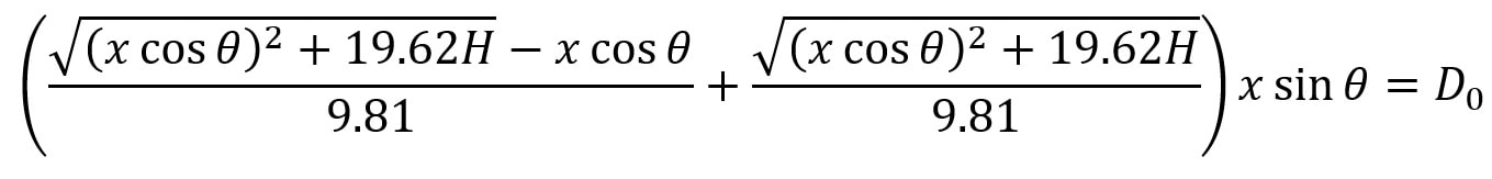
We can now subtract the length of the table (2.74m) from D0 to give the distance in metres the player should stand from the table to hit the optimum lob shot. (D1) 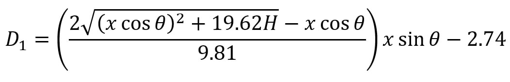 This shows us some of the ways that mathematics can be used to help sports players. You can find a more detailed analysis of the maths involved in the table tennis lob shot here. For suggestions or feedback, please write to [email protected].
Nitya Nigam Internet privacy is an important and relevant issue in today’s world, especially given recent moves by world governments to restrict the influence of foreign technology companies in their countries. This is why Integral has partnered with Bytesized Privacy to give our readers insight into encryption, one of the most effective ways to ensure private data stays private. This article will cover the maths behind the Diffie-Hellman key exchange, which is a secure and widely used method of public key cryptography. Bytesized has a post about the applications as well as the pros and cons of end-to-end encryption that you can find here. We hope you find this collaboration useful and interesting. Let us know in the comments if you’d like to see more posts like this!
Public key cryptography is a type of encryption where each person has a pair of cryptographic keys: a public key and a private key. The private key is kept secret, but the public key can be used by anybody. The Diffie-Hellman key exchange uses public and private keys to give both sender and receiver a shared key that can be used in future communications, as the process of using both public and private keys for every message is computationally expensive. The maths behind this key exchange is based in modular arithmetic, where integers that have the same remainder when divided by a set integer are considered the same, or “congruent”. We can notate this mathematically by saying that, for example, 6 ≡ 1 mod 5, where the ≡ symbol means “congruent to”, mod means modulo (x mod y means x is the remainder when a number is divided by y) and 5 is the set integer we are using as the base of this system. The Diffie-Hellman key exchange involves 5 steps, outlined below. Let our two people who want to communicate with each other be called Alice and Bob.
Alice and Bob now have a shared key, s, that they can use for secure communication, that is unknown to all other users. This method works because B ≡ g^b mod p and A ≡ g^a mod p, so B^a ≡ g^ba mod p and A^b ≡ g^ab mod p, which are equivalent. This method is secure because for large p, a and b, reversing the modular exponentiation is near-impossible via a brute force attack, because there are many different possible values of base and exponent that lead to the same value after reducing the result mod p. g is usually quite small, as most primitive roots are small integers like 2 and 3. g being small does not compromise the security of the system. Malhar Rajpal As seen in my previous article (reading it will help you understand this article), Minimax is a fantastic way to program game engines so that they play effectively. However, for more complex games, like chess, Minimax would take far too long to find the optimal move, even if it’s only looking 4 or 5 moves ahead! This speed problem, however, can be easily resolved with alpha-beta pruning. Alpha-beta pruning is a search algorithm that explores less nodes (triangles) than Minimax does while still outputting the same best action for the player. It does this by evaluating the score of one node from a group of previous nodes at a time (similar to Minimax). However, upon evaluating the score of another node, if the output score is proven to be worse than other previously explored output scores before some of its child nodes are even considered, then the program doesn’t bother exploring these child nodes, therefore saving time. In other words, it returns the same move as Minimax while removing (or pruning) irrelevant nodes before they are examined. This sounds very complex but I assure you that after you read the example, you will find that it is actually a very simple concept! Let’s take a look at a Minimax diagram similar to the one shown in my Minimax article in which each player has three possible choices. I have given arbitrary values for each of the 9 possible outcomes resulting 2 actions ahead from the initial move (or root node). 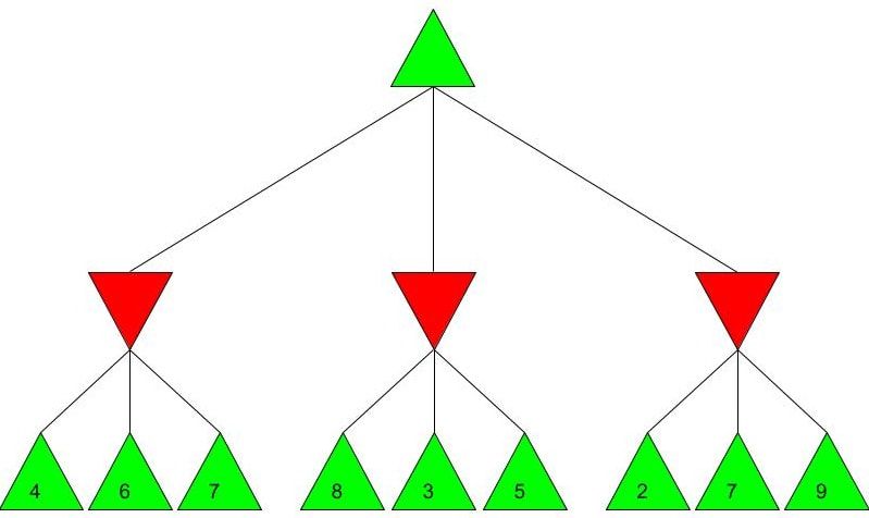 For the first minimizing node (triangle) from the left, we can do it the same way as we did using Minimax. Since the minimizing player will always choose the lowest possible option (since it is playing optimally), out of the possible scores of 4, 6, 7, the minimizing player will choose 4, as shown in the diagram below: 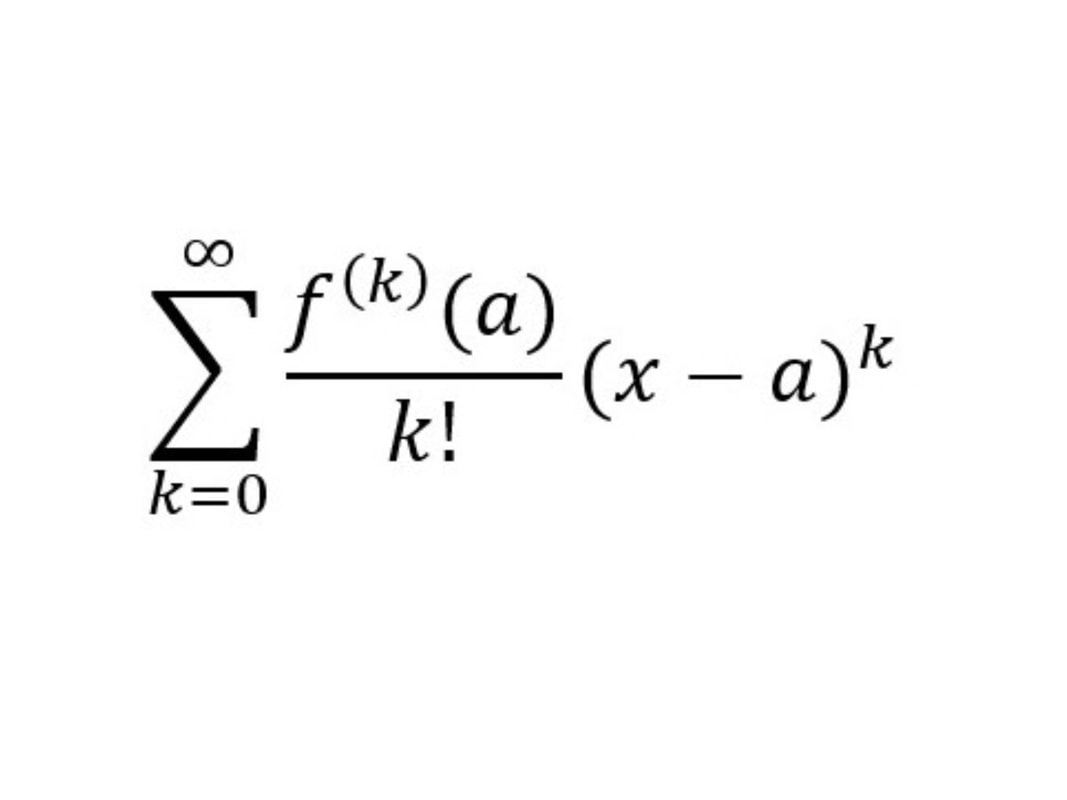 This is the exact same as Minimax! But for the middle minimizing node, the algorithm first explores the child node with a score of 8, then the node with a score of 3. Since 3 is less than 8, and it’s the minimizing player’s turn, the algorithm will prefer the node with the score of 3. We can also, however, see that 3 is less than the 4 from the leftmost minimizing node. This means that even without considering the node with value of 5, we can say that the middle minimizing node must have a score that is less than or equal to 3(<=3), since the minimizing player will always choose the lowest possible score. We don’t need to consider the node with value of 5 because the node with a score of 4 from the left is greater than the already explored node with score 3, hence for the root node, the maximising player will prefer the node with score 4 over the score of the middle node which can be said to be <= 3. In other words, there is no possible score for the node coloured blue below, that would change the decision of the root node. 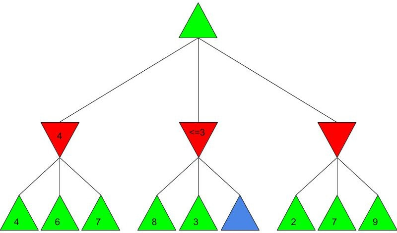 We, therefore, can prune the node coloured blue and any potential nodes that branch below it, hence saving a lot of time! I put <=3 in the middle minimizing triangle for clarity, however the program will not need to consider it when evaluating the score for the root node since the maximising player always prefers the node with a score of 4 over the <=3 score in the middle minimizing triangle, so we can just eliminate this branch entirely. Now we can calculate the rightmost minimizing triangle. Immediately we see a node with the score of 2. So we can immediately say that the rightmost minimizing node must have a score of <=2 (since the minimizing player will always choose the lowest score). Since the next move, made by the maximising player, will always prefer the score of 4 in the leftmost minimizing node over the <=2, we don’t even need to consider looking at the nodes with scores of 7 and 9. Eliminating these nodes and the nodes that could branch off below them without even exploring them saves even more time! 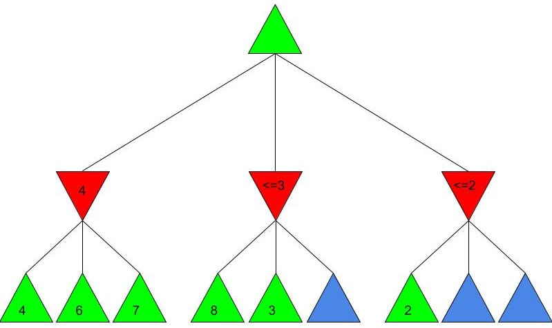 When we prune a node, that means that we don’t need to consider its parent node either. We can therefore eliminate that entire branch too, since if a child node is pruned, its parent node will not be preferred as compared to one of its aunt/uncle nodes. So when we prune the sixth, eight and ninth nodes from the left, we can subsequently eliminate its parent node too: 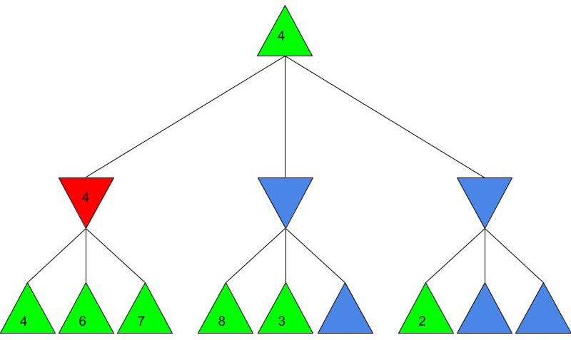 Now since the root node only needs to consider the node with value 4, it will be chosen (as shown above) without even considering the other nodes, further cutting down on algorithm runtime. If you were to try and evaluate the Minimax tree as we did in the previous article, you would find that the score in the root node would be the same. The only difference would be that, when programmed, the alpha-beta pruning algorithm would take substantially less time.
Alpha-beta pruning is a powerful algorithm that can be used to program game engines in an even more efficient manner. When used with depth-limited Minimax, alpha-beta pruning can be used to make engines quickly play near-optimal moves in games as complex as chess! Nitya Nigam The global COVID-19 pandemic continues to rage on, with the total number of cases around the world having just hit 13 million. In addition to mask-wearing and social distancing, scientists have highlighted widespread testing as an important measure in reducing the spread of the coronavirus. However, many regions do not have sufficient equipment and chemicals to run individualised tests. For this reason, the mathematical strategy of group testing has been suggested as a way to quickly test a large number of patients without using up an excess of precious testing materials. Group testing involves mixing samples of several people together, and then testing the mixture in one go. If this test comes back negative, then all of the people whose samples went into the mixture are marked as negative at once, saving time and resources. However, if this test comes back positive, further testing is required to pinpoint the infected individuals. There are four main techniques to do this. 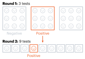 Method 1 involves samples being mixed together in groups of equal sizes, and then these mixtures are tested separately. If a group tests positive, then each individual member of the group is retested. This method was used in Wuhan, China in May, as part of efforts to test the majority of the city's population, identifying 56 infected people from about 2.3 million individuals involved in testing. This method works best in low levels of infection (about 1% of the population), because group tests are likely to be negative. 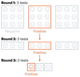 Method 2 is a more sophisticated version of Method 1, which adds more rounds of group tests before testing individuals separately. However, both of these approaches are quite slow, as it takes several hours to get the results for each group test. These group results must be known before further testing can occur to pinpoint individual infections. “This is a fast-growing, fast-spreading disease. We need answers much faster than this approach would allow,” says Wilfred Ndifon, a theoretical biologist based in Rwanda. 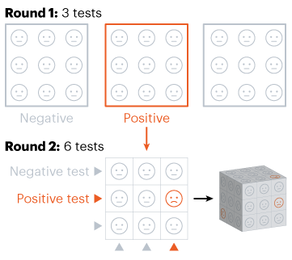 Ndifon and his colleagues at the African Institute for Mathematical Sciences have improved on these strategies, aiming to reduce the number of tests needed. Their first round of group tests is the same as described above, but for positive-testing groups, they propose a different method. Imagine a 3x3 grid, where each cell represents one person’s sample. The samples in each row and column are tested as one group, meaning there will be 6 total tests, and each individual will have been tested twice. If an individual sample is positive, it will cause both groups it is part of to be positive, making it easy to find the individual. The dimensionality of testing can be increased from a square grid to a cube, which allows for bigger groups and higher efficiency. This constitutes Method 3. 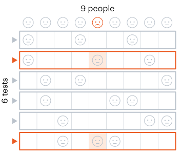 Although Method 3 decreases the number of tests that must be conducted, some scientists say that even two rounds of testing take too much time. Manoj Gopalkrishnan, a computer scientist at the Indian Institute of Technology Bombay, has proposed a one-step solution that is our Method 4. His approach involves mixing samples in different groups, using a counting technique known as Kirkman triples, to determine how the samples should be distributed. Imagine a grid in which each row represents one test, and each column represents one person. In general, each test should have the same number of samples, and each individual’s sample should be tested the same number of times. This method requires more tests to achieve the same level of accuracy as the previous methods and also means working with a large number of samples at once. However, it significantly decreases the amount of time taken to test a large group of people.
Let us know in the comments if you enjoyed this article, and what your thoughts on group testing are! |