|
Malhar Rajpal Imagine you have a complex maze with hundreds of ways to reach the endpoint. How do you find the shortest route? This is the exact problem that appears in a vast array of real-world problems from GPS navigation to tracing garbage collection. You could split the problem into an unweighted graph, where each position in the maze or street on the map is a node, and try to manually trace the different solutions from the initial position (also known as the root node) to the solution. But you will soon find that, since there are so many different routes, solving this problem manually is a near-impossible task! You need to use a computer algorithm, and luckily for you, the solution comes in the form of Breadth First Search (BFS), which explores each node in the unweighted graph until the solution is reached. To explain the concept of BFS, I will use a basic example: 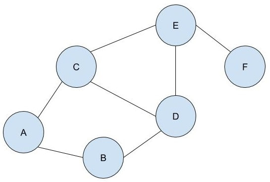 L circle (node) A be our root node, and we must traverse our way to node F, which is our end node, or solution. We could analogise each of the nodes in the graph to be a certain street, and each of the lines show which streets are connected (for example street A is directly connected to street B or street C). There are obviously several ways to get from node A to node F (two of which could be A → B → D → E → F or A → C → D → E → F), but we want to get to node F by traversing through the least amount of nodes or streets. How would the algorithm do this? The answer is not as complex as you may think. The algorithm requires a list (more formally called a frontier). This frontier contains the nodes that are currently being explored. Another list is also needed which contains the explored nodes. When the algorithm initialises, node A (our first node) is put into our frontier (as shown below) since it is the first to be explored. The list containing the explored nodes remains empty. 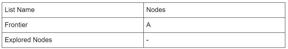 The frontier makes use of a queue data structure which, simply put, will always explore the first node that was appended in a list (in this case our frontier). Since node A is our only node, and hence the first node, it is explored. The exploration process includes checking if the current node is equal to the solution node. If it is, then the program can return the path needed to reach the final node. If not, the program will check if any of the directly connected nodes to the current node is in the ‘Explored Nodes’ list. The program will then simply add all the connected nodes that are not in the ‘Explored Nodes’ list to the frontier. So in our example, since node B and C are directed connected to A, and since neither node B or C are in the explored nodes list, they are both added to the frontier like so: 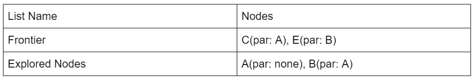 Since node A is now explored and a queue is a first in first out data structure, meaning the first node in the list is the node that is removed when needed (when a node is removed from a queue, it can only be the first first node in the list). Node A is then added to the explored nodes: 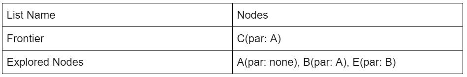 Each node contains the needed data (street name etc.) as well as the parent node within itself. For example, node B contains its own information as well as its parent element (node A). These parents will be labelled in our table using the format ‘par: letter of node’. Now, since node B is the first node in our frontier, it follows the same process as before: it is checked whether it is the solution node (node F). Since it’s not, the program gets all its connected nodes: node A and node D. Since node A is already explored, it is ignored (this avoids backtracking) and node D (with its parent being node B) is added to the frontier. Node B is then added to the explored nodes. 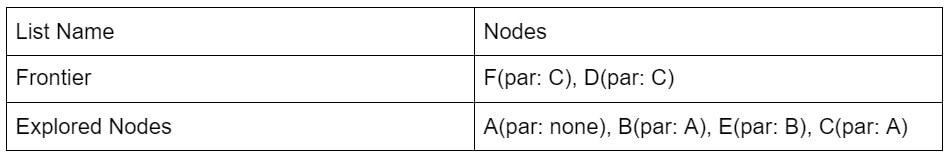 This process is continued until we arrive at the following table: 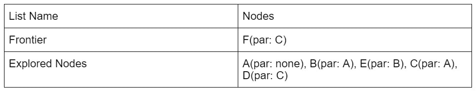 Finally node F is our solution. Since we kept track of the parents, we can easily backtrack the optimal route from the solution node (Node F) all the way to the initial node. We can do this by creating a list and adding the subsequent parent elements of each of the previous nodes to the list, until we reach node A (which has par:none). This gives us this list: (F, E, C, A). Reversing this list, we can find the shortest route to node F: Node A → Node C → Node E → Node F (shown in red on the below diagram), which only traverses through four nodes! This is great since our programs can easily perform each exploration in a matter of milliseconds, allowing incredibly complex search problems to be entirely solved in as little as a couple of seconds! 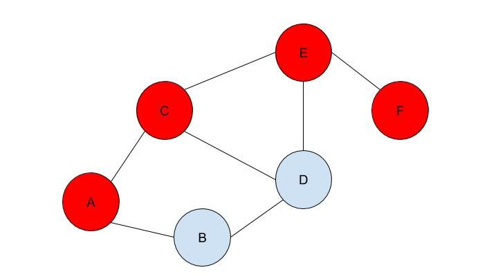 BFS is a widely used algorithm, effective in finding the shortest route from one node to another. Although complex problems like GPS navigation systems use slightly different algorithms since they must take into account several different aspects (traffic, speed limits etc.), these algorithms are all built upon the fundamental principles of BFS. If you want to go deeper into the world of search algorithms, I would suggest looking at A* search, which finds the route between two nodes with the lowest cost (cost referring to some variable; it could be lowest time, lowest distance etc.).
0 Comments
Leave a Reply. |