|
Nitya Nigam If you keep up with the latest developments in mathematical research, you may have heard the term “topology” being thrown around, but might not know exactly what it is. Topology is a branch of maths that studies the properties of spaces that stay the same after continuous deformation. In topology, objects can be stretched and squeezed like rubber, but they cannot be broken, so it is sometimes called “rubber-sheet geometry”. Under these rules, a triangle can be deformed into a circle, but the number 8 cannot, as it has two holes in it. So, circles and triangles are topologically equivalent, but are distinct from figure 8s. In honour of Maryam Mirzakhani’s birthday (the first woman to win a Field’s Medal, awarded to her for her groundbreaking research in topology), I thought I would write an article about one of current mathematics’ most active research fields. Links to relevant external resources are provided throughout the article in case you would like to extend your knowledge. You may wonder why topology is relevant. It has only emerged as a distinct mathematical field relatively recently; most topological research has been done after 1900. However, graph theory, which studies the properties of spaces built up from networks of vertices, edges and faces, is a form of topology. Spaces in graph theory are considered identical if all the vertices are connected up in the same way, regardless of their layout; graphs which are structurally identical but are laid out differently are called isomorphic, and are topologically equivalent. Graph theory has a wide range of applications in computer science, such as modelling computer networks, but it can also be used to optimise road networks and analyse linguistic trends. Nonetheless, the modern topological research goes far beyond graph theory, and has applications in branches of physics like vector fields and string theory. One main subfield of topology is point set topology. It analyses the local properties of spaces, and is closely related to calculus. It generalises the concept of continuity from calculus to define topological spaces, so the limits of sequences can be considered. If distances can be defined in these spaces, they are called metric spaces. In some cases, the distance cannot be defined - if a space maintains its continuity after a deformation is applied, it is still fundamentally the same space, but its “size” will have changed, so the concept of distance makes no sense. Another area of topology is algebraic topology, which instead considers the global properties of spaces. It answers topological questions by converting topological spaces into algebraic objects such as groups and rings. For example, topological spaces like the torus and the Klein bottle, pictured below, can be distinguished from each other because they have different homology groups (an algebraic concept based on integrating surfaces). Similarly, other algebraic concepts can be used to analyse and research topological spaces. 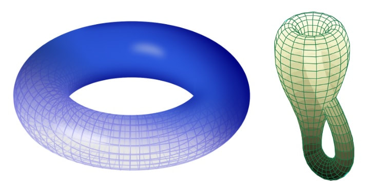 The final area of topology discussed here is differential topology, which studies spaces with some kind of smoothness associated with each point. In this field, the triangle and circle would not be equivalent to each other in terms of smoothness - the triangle has hard corners, whereas the circle has a continuously curved edge. Differential topology is particularly relevant in vector field physics, and is therefore used to study things like magnetic and electric fields. It is also helpful in describing the 4-dimensional space-time structure of our universe.
This is just an overview of the immensely complex and constantly evolving field of topology. If this article sparked your interest, you can follow the latest mathematical research explained simply at ScienceDaily. Let me know in the comments what parts of topology you find particularly intriguing, and what you’d like to read about next!
0 Comments
Nitya Nigam Machine learning is a buzzword that has been plastered across the media for the last few years. With applications in any field you can think of, it has been touted as a technology that can revolutionalise the way we work and think. To a large extent, this is true: machine learning is used in everything from Covid-19 infection modelling to giving you personalised Netflix recommendations. Many people are under the impression that the way machine learning operates is too complicated for the average Joe to understand. However, the underlying principles of machine learning are actually quite straightforward. In this article, I will outline the intuition underpinning machine learning, and explain some of the maths required to make it work. All concepts that may be new to our readers are linked to an external resource to help build understanding.
In essence, machine learning is a computerised method of finding models for data. Machine learning algorithms work by:
In step 1, a polynomial function is generated to model the data. Although not all situations can be modelled perfectly by polynomial functions, exponential, logarithmic and trigonometric functions can all be represented as polynomial functions through their Taylor series representations. Essentially, through a funky bit of calculus (3Blue1Brown does a nice explainer of this on his YouTube channel), we can show that these functions are the infinite sums of polynomial series. Obviously, we can’t use an infinite number of polynomial terms in our function, but we can use a large amount, and this is often more than enough to properly model data within a given domain. The coefficients of the polynomial terms, or parameters, are stored in vectors, with one vector for each of the input variables. These parameter vectors will be what we change in order to improve the model, so keep them in mind. Step 2 makes use of something called a cost function. This measures the average distance between each value in the test data and the value predicted by the model. Usually, the measure used is the variance, which is a statistical measure of dispersion. The reason this is used, as opposed to the difference, is because it is squared, so values that are too high and too low both increase the variance, rather than cancelling each other out. The process of computing the variance of the data is called the cost function, and the output of the cost function for a given set of model parameters is a scalar value. When the cost function is high, this means the model does not fit the data well, so steps must be taken to increase the accuracy of the model and decrease the cost function. Step 3 is where the magic really happens. Through a bit of differential calculus, we find the gradient (also known as the slope, derivative or rate of change) of the cost function, which is a function of the model’s parameter vectors. This means that as the parameters change, the cost function will also change. When the gradient is negative, this means the cost function is decreasing, so taking a step in that direction would bring us to a lower cost and a more accurate model. Taking small steps in the direction of the negative gradient is called gradient descent (the method is explained further in this video), which eventually lands us in a spot where the gradient is zero, and is a minimum of the function. The values of the parameter vectors at this point should be optimised for the data we are trying to model. This is just an overview of what constitutes machine learning - there are several issues not covered here, such as how to avoid local minima and optimising step size, but I hope this serves as a helpful introduction to the topic. Let me know if you want to learn more about maths in machine learning in the comments! |