|
Nitya Nigam If you follow tennis, you've probably seen matches where games stretch into a sixth or seventh deuce, seemingly going on forever. Theoretically, if players alternated winning points from deuce, a game could last ad infinitum - the current record is 37 deuces, set in 1975. In this article, we'll find the probability that player A wins a game of tennis from deuce, given that the probability they win a point is p. This is an obvious simplification, as the probability of a player winning a point would not stay the same throughout a match, but it makes things clear in terms of the maths. For our readers who are unfamiliar with the tennis scoring system, you can find a clear and concise guide here. Firstly, let us define some probabilities. Let P_D be the probability that player A wins given that the game is at deuce. Let P_Ba be the probability that player A wins given that player B is at AD. Let P_Aa be the probability that player A wins given that player A is at AD. Now, we can use conditional probability rules to find three equations in terms of these three probabilities and our base probability p, allowing us to solve for P_D. P_D = (prob. A wins first point)(prob. A wins from AD) + (prob. B wins first point)(prob. A wins from B at AD). The probability A wins the first point is just p, so the probability B wins the first point is 1-p. Therefore: P_D = p P_Aa + (1-p) P_Ba The conditional probability equation states that P(A|B) = P(A and B) / P(B), where P(A|B) refers to the probability of event A occurring given that event B has already occurred. In our case, P_Ba = P(A wins point | B at AD) = (p x (1-p) x P_D) / (1-p) = p P_D. Similarly, P_Aa = P(A wins point | A at AD) = (p x p x P_D) / (p) Substituting these into our equation for P_D gives: 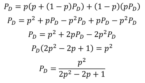 When we graph this equation, we get the following shape: 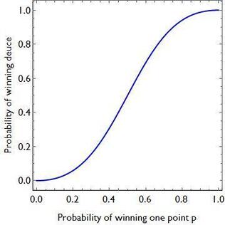 The shape of this graph is quite interesting. When p is 0.5, the probability of winning from deuce is also 0.5, so chances are even. But if p differs even slightly from 0.5, the chances of winning from deuce increase or decrease quite significantly. The shape of this graph demonstrates that players need to have very similar point probabilities for a game to be close. Given that so many matches in today's climate are very close, this shows just how close to each other the players are in ability, and how even a slight edge can have huge consequences.
Let us know in the comments if you were interested in this article about maths in sports, and tell us what you'd like to read about next!
0 Comments
Malhar Rajpal Most math competitions have stringent time limits and a prohibition of calculator use. Because of this, it is extremely important to learn basic strategies to perform quick mental calculations to solve more problems and thus be more successful in such competitions. Furthermore, performing mental math in front of a live audience is extremely impressive: imagine squaring huge numbers in your head quicker than any calculator can do it! In this article, you will learn the strategy of quickly squaring two digit numbers and the reasoning behind the method.
Squaring a two digit number in your head: Imagine seeing 56x56 on your exam paper, as you’re scramming for time. It would be a huge pain to calculate this using table multiplication and you would save at least half a minute by doing this in your head. How would we do this? The method: If we take any two digit number, say in this case we take 56, we first round it to the nearest 10. So if our number is 56, we round to 60. If our number is 42, we would round to 40. Then you find the difference between the rounded value and the initial value. So 60-56 = 4 or 42-40 = 2 and you perform the “reverse calculation” by that same value: If you initially chose 56, you have to add 4 to get 60, and hence the reverse calculation would be to subtract 4, and this number would be 56-4 = 52. If you had to square 42, you subtract 2 to get 40, and hence the reverse calculation would be to add 2 to get 42+2 = 44. After you get the two numbers, the rounded number and the number you obtained after performing the reverse calculation, you multiply them together. So for squaring 56, you would multiply 60 and 52, which is just 6x10x52 = (6x52)x10 = 3120 and for squaring 42, you would multiple 40 and 44, which is 4x10x44 = (4x44)x(10) = 1760. After you have this number, you take the difference between the rounded number and the initial value that you found before and square it. So for 56, 60 is the number rounded to the nearest 10 and 60-56 = 4. We take 4 and square it to get 16. For 42, 42-40 = 2, so we take 2 and square it to get 4. After we get this squared value, we add it to the product that we calculated(the product after multiplying the rounded number and the reverse calculation number). So for 56, we have 3120+16 = 3136, and for 42, we have 1760+4 = 1764, which are our final answers! Amazing how simple it is, isn’t it! It’s simpler than trying to do it manually because you are essentially multiplying a two digit number with a multiple of 10(which is the same as multiplying a two digit number by a one digit number and then multiplying the product by 10), and then adding a small number to that result to get the final answer. Let’s try one more example: 73. 73 rounded to the nearest 10 is 70. 73-3 = 70, hence the reverse calculation is to add 3 to 73: 73+3 = 76. We then multiply 76 with 70 which is the same as 76x7x10 = 532x10 = 5320. The difference between the rounded number, 70, and initial number to square, 73 is 3, and 3 squared = 9. We, thus, add 9 to our existing product to get: 73x73 = 5320 + 9 = 5329, our final answer! The mathematics and reasoning behind the method: The mathematics behind this method is actually very simple. Let’s say we have a number, a. We want to find a^2. By the method, we are adding or subtracting some value b from a to get the rounded value. We then perform the reverse operation subtracting or adding b from a. Finally we multiply these two numbers together and this can be represented as: (a+b)(a-b) where the first number is the rounded up value, and the second number is the number after performing the reverse operation on a. We could also have (a-b)(a+b)if the rounded number is rounded down instead of up, however, since xy =yx, (a+b)(a-b)=(a-b)(a+b) hence both expressions are equivalent. After we evaluate the product (a-b)(a+b), we add the value of b^2 to the product to obtain our final answer. We can thus hypothesise that a^2=(a-b)(a+b) + b^2 and now we have to prove this. The proof is direct and just requires an expansion of the right side: a^2=a^2-b^2+b2 and the b^2s cancel out leaving us with a^2=a^2, an equivalent statement so we know that a^2=(a-b)(a+b)+b^2 is true and our methodology therefore works for any real a and b! Nitya Nigam Since the advent of modern computing in the 1950s, computers have played an essential role in mathematical research. They're often used to test conjectures, as they can iterate through long lists of numbers extremely quickly to check whether they satisfy the conditions that have been predicted. They are also used to find specific types of numbers, such as Mersenne primes (you can even join the Great Internet Mersenne Prime Search yourself). However, coming up with conjectures has long been the work of mathematicians themselves. A good mathematical conjecture states something profound and useful within the field. It must be interesting enough to prompt investigation, but not so niche as to have very narrow applications. Getting computers to strike this balance is therefore a tall task.
However, researchers at the Technion in Israel have created an automated conjecturing system called the Ramanujan Machine, named after the famous mathematician Srinivasa Ramanujan. The software has already conjectured original formulas for several mathematical constants (published in this Nature article) including Catalan's number and pi. The software works by leveraging the fact that many such constants are equal to continued fractions (fractions where the denominator is the sum of two terms, one of which is a fraction with a denominator that also contains a fraction, and so on until infinity). Continued fractions have been of mathematical interest both for their aesthetics and what they reveal about constants' fundamental properties. The software works by first finding continued fraction expressions that seem to equal universal constants by choosing arbitrary constants and expressions, then computing each side to a certain level of precision and seeing if they approach each other. If they seem to approach each other, they are computed to higher precision to ensure that it is not a coincidence. Since formulas already exist to compute pi and other constants to an arbitrary level of precision, the only thing in the way of making sure the sides match is computing time. So far, the software has conjectured a formula for Catalan's constant that allows for its fastest computation yet. This is an important milestone for computational mathematics, not just because it shows promise for developing faster methods to compute other constants, but because these automated conjectures may be used to reverse-engineer more theorems, further fueling mathematical innovation, Malhar Rapal While studying for a math competition, I encountered Brahmagupta’s formula, which states that the area of any cyclic quadrilateral (all vertices of the quadrilateral lie on a single circle) is equal to: 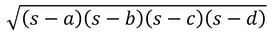 where a, b, c, and d are the 4 side lengths of the quadrilateral and s is the quadrilateral’s semi-perimeter: (a + b + c + d)/2en.wikipedia.org/wiki/Heron%27s_formula. I was astounded by its similarity to Heron's Formula for triangles as well as Bretschneider's formula and wondered why Brahmagupta’s formula stood true for all cyclic quadrilaterals. In this article, I will derive Brahmagupta’s famous formula. 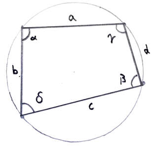 Note: All angles in this article will be referred to in degrees. The diagram above depicts a cyclic quadrilateral with sides a, b, c, d and angles α, β, γ, and 𝛿. One property of cyclic quadrilaterals is that all opposite angles are supplementary. This means that α + β = 180, and γ + 𝛿 = 180. Using α + β = 180, we see that α = 180 - β and thus by apply cosine on both sides: cos(α)=cos(180-β). The difference formula for cosine states that cos(a-b) = cos(a)cos(b) + sin(a)sin(b) for any a and b. We can use this formula on cos(180-β)to get: cos(α) = cos(180)cos(β) + sin(180)sin(β). cos(180)= -1 and sin(180)=0 hence cos(α) = -cos(β). We also apply sine to both sides to get sin(α)=sin(180-β). The difference formula for sine is sin(a-b) = sin(a)cos(b) - sin(b)cos(a) hence sin(α)=sin(180)cos(β)-cos(180)sin(β). sin(180) = 0 and cos(180) = -1, hence sin(α)=sin(β). 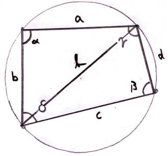 Now, we can split the cyclic quadrilateral into two triangles as shown above with a diagonal of length L. We can use cosine rule for triangles which states that a^2=b^2+c^2 - 2bc cos(A) for triangles with side lengths a, b, c and an angle A opposite to side a. One triangle is bounded by sides a, b, and L and the other triangle is bounded by c, d, L. By applying the cosine rule on both of these triangles, we can see that L^2=a^2+b^2-2abcos(α)and L^2=c^2+d^2-2cdcos(β). We can therefore state that for this cyclic quadrilateral, a^2+b^2-2abcos(α) = c^2+d^2-2cdcos(β) Since cos(α)=-cos(β), we can say that cos(β) = -cos(α). By replacing the occurrence of cos(β) with -cos(α) in the equation a^2+b^2-2abcos(α) = c^2+d^2-2cdcos(β), we get: a^2+b^2-2abcos(α) = c^2+d^2+2cdcos(α) . And by simple rearrangement and factoring: a^2+b^2-c^2-d^2=2cos(α)(ab+cd). Now, we can use the area of the two triangles to get the area of the entire cyclic quadrilateral. Since Area = 1/2 ab sin(C)for a triangle with sides a, b and angle C opposite to the third side (side that’s not a or b), we can see that the area of the triangle bounded by a, b, and L is 1/2 ab sin(α) and the area of the triangle bounded by c, d, and L is 1/2 cd sin(β) . Since the entire cyclic quadrilateral is composed from these two triangles, the area of the quadrilateral is the sum of the areas of the two triangles. Thus, we state that A = 1/2 ab sin(α) + 1/2 cd sin(β). Using sin(α)=sin(β), we replace sin(β) with sin(α)and rearrange to get A=(ab+cd)/2 sin(α) . And by making sin(α) the subject, we get sin(α)=2A/(ab+cd). Brahmagupta faced a problem. How could he relate sin(α)=2A/(ab+cd) with a^2+b^2-c^2-d^2=2cos(α)(ab+cd)? Since for any right angled triangle the sine of an angle is the opposite/hypotenuse and since sin(α)=2A/(ab+cd), the proof creatively formulates a right angled triangle as shown above with hypotenuse ab+cd, a side 2A opposite to an angle α. By using the Pythagorean theorem, the third side becomes: 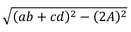 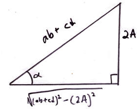 With any right angled triangle, cos(a)= adjacent/hypotenuse. Thus: 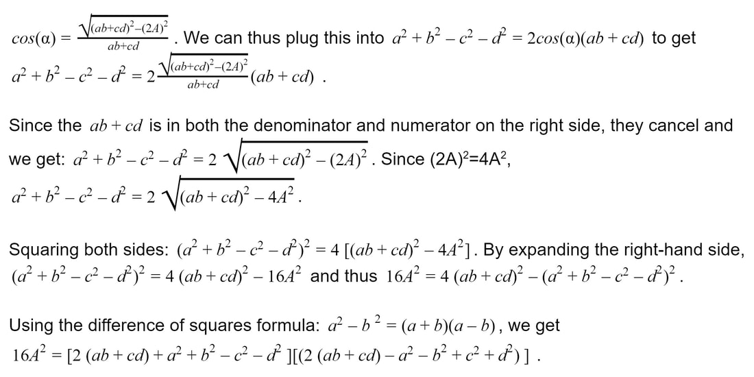 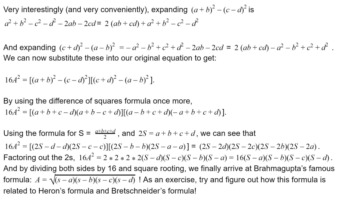 Nitya Nigam A lot of competition maths problems involve finding ratios of areas of various shapes, so having a quick way to find them is a useful tool. In this article, we'll derive the following equation for the area of a regular polygon: 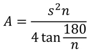 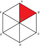 where s is the side length and n is the number of sides. To get to this equation, we first need to consider one of the n triangles that make up the polygon, one of which is shown in red on the right. The central angle of this triangle will be 360/n for any n-sided regular polygon.  The green angle is 360/n, as stated above, so the orange angle θ is half of that, so θ = 180/n. tan θ = (s/2)/h so h = s / (2 tan θ). The area of a triangle is 1/2 of its base times its height, so the area of this triangle is 1/2 * s * s / (2 tan θ) = s^2 / (4 tan θ). We can then substitute θ = 180/n in, giving A_(triangle) = s^2 / (4 tan (180/n)).
Since there are n of these triangles in an n-sided regular polygon, the total area of the polygon is n * A_(triangle) = n s^2 / (4 tan (180/n)), as above. Malhar Rajpal In physics, a capacitor is a device that stores electrical energy. A capacitor is made up of two plates with a dielectric material between the plates. When a voltage is applied to a circuit with a capacitor, positive charge builds up on one plate while negative charge builds up on another plate, with the result being a potential difference (potential refers to the electrical potential as a result of the different charge between the plates). When the potential difference of the capacitor is the same as the voltage applied in the circuit, the current in the circuit becomes 0 and the capacitor’s p.d. stops increasing. The ‘charging’ process for the capacitor happens very quickly when there is no resistance in the circuit. If there is a resistance, by I=V/R, the current is lower and thus the charge builds up slower on the plates, slowing down the charging process. The more resistance, the slower the capacitor reaches the voltage applied. A capacitor also has a property called capacitance, C, which is the ratio of the amount of electric charge stored on a conductor to the difference in electric potential (this is directly proportional to the area of the plates and inversely proportional to the distance between the plates). The maximum charge on a capacitor is given by the equation Q = CV, where Q is charge, C is capacitance, and V is voltage. The capacitor can then be removed from the circuit with the power source and put in another circuit without a power supply. The charge then dissipates from the capacitor and flows through the circuit. This causes the absolute value of the charges on the plates and therefore the potential difference to decrease until they reach 0. The rate that the charge decreases with time of some capacitor with capacitance C depends on the resistance of the circuit and today we will explore the mathematical model finding the charge Q in this circuit at any given time while the charge dissipates. In the new loop, with the capacitor and some resistance, R, the current I of the circuit can be modelled by: I=V/R and V=IR. From above, we have the equation linking charge to capacitance and p.d.: Q = CV. Rearranging this equation, we see that V = Q/C. Substituting V = IR, IR = Q/C and thus I=Q/(RC). Current is also defined as the net rate of flow of electric charge, which can be defined mathematically as the change in charge over the change in time: ΔQ/Δt. Since charge is being dissipated (decreasing), we can say that ΔQ/Δt must be negative and, being physicists (this step is illegal is maths!), we can can say that I = -ΔQ/Δt. Now that we have two expressions for I, we can combine them: -ΔQ/Δt = Q/(RC), a differential equation! Using calculus notation, -dQ/dt=Q/(RC). Rearranging this equation, we get (1/Q)dQ = -1/(RC) dt. We can now integrate both sides: 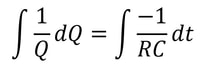 Since we don’t want the unknown constants resulting from indefinite integration in our final expression, we need to make both integrals definite (along a fixed range). We can say that we start at t=0 and go until t=t. When t=0 seconds, Q = Q_0 (initial capacitance), and when t=t seconds, we can say that Q=Q (some capacitance). So we get: 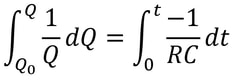 Solving this, since -1/(RC) is a constant with respect to t, we can bring it out of the integral to get: 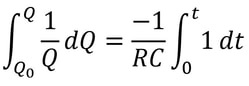 The indefinite integral of 1/Q dQ is just ln(Q) + C (natural log of Q), where C is an arbitrary constant, so by using the definite integrals, the left side of the equation is: 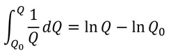 The indefinite integral of dt is just t+c and thus the right side becomes: 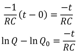 Using ln(a) - ln(b) = ln(a/b), ln(Q) - ln(Q_0) = ln(Q/Q_0). We can now raise e (Euler’s constant) to the power of both sides to get:  Since e^(ln(a)) = a for any a, we can rewrite as Q/Q_0= e^(-t/(RC)) and thus:  where Q is charge, Q_0 is initial charge, e is Euler’s constant, t is time since discharge begun, R is resistance, and C is capacitance.
The units of RC is seconds and it is thus be referred to as the time constant, τ. Using Q=Q_0 e^(-t/(RC)), when t = τ, Q = Q_0/e; when t = 2τ, Q = Q_0/e^2; when t = 3τ, Q = Q_0/e^3. In every discharge cycle, the time constant is equal to the amount of time taken for the charge to reduce to ~37% (1/e) of its initial value. Since charge is easily measured and this time is a constant, one great use for capacitors is in timing circuits! As an exercise for yourself, try showing that the equations V=V_0 e^(-t/(RC)) and I = (V_0 / R) e^(-t/(RC)) also hold true in RC circuits! Nitya Nigam There are four recognised types of conic sections: circles (probably the most familiar of the lot), ellipses, parabolas and hyperbolas. You’ve probably encountered the equation of a circle: (x-h)^2 + (y-k)^2 = r^2, where (h, k) is the circle’s centre, and r is its radius. In this article, we’ll derive the equations for ellipses and parabolas. Parabolas are defined as curves such that all points on the curve are equidistant from a point, called the focus, and a line, called the directrix. The diagram below displays this clearly: 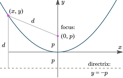 We can see that the vertical distance d from point (x, y) to line y = -p is y + p We can also see that the distance d from point (x, y) to the focus (0, p) is sqrt(x^2 + (y-p)^2) Equating these distances and rearranging gives the following: 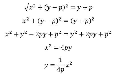 This is the standard equation for a parabola centred at (0, 0). As with the circle equation, we can shift parabolas around by incorporating the parameters (h, k) into the equation like so: 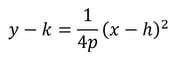 And that is the parabola equation! Ellipses are defined as curves such that, for all points on the curve, the sum of the two distances to the two defining “focal points” is constant, and this sum is equal to the length of the major axis, which is the longer distance between the two “vertices” of the ellipse. This diagram provides a visual explanation: 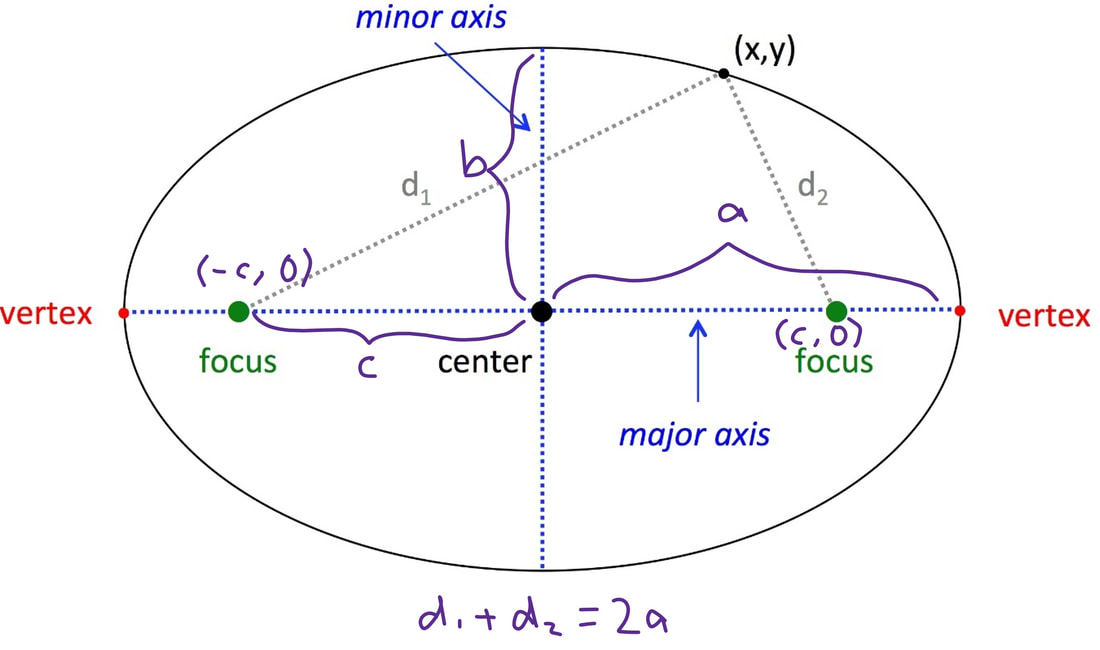 By Pythagoras’ equation, d_1 = sqrt[(x + c)^2 + y^2] and d_2 = sqrt[(c - x)^2 + y^2]. By applying this to the point (0, b) we obtain d_1 = d_2 = sqrt(c^2+ b^2). Substituting this into d_1 + d_2 = 2a gives: 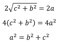 Using this information, we can use the general expressions for d_1 and d_2 to find an equation involving only x, y, a and b. 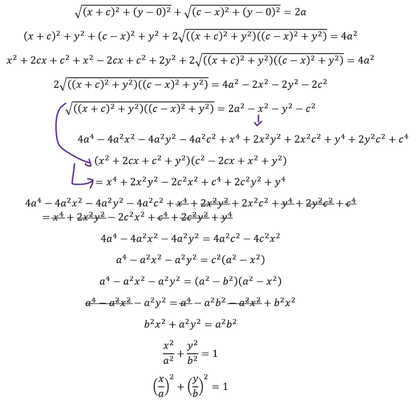 This is the standard equation for an ellipse centred at (0, 0). As with the circle and parabola equations, we can shift ellipses around by incorporating the parameters (h, k) into the equation like so: 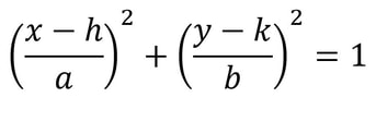 And that is the ellipse equation!
Let us know in the comments if you found these derivations useful, and what you'd like to see next! Nitya Nigam Readers who study physics may have encountered the small angle rule in their classes. It's an essential tool in simplifying equations, both at a high school level and beyond. But what is the rule? You're probably familiar with the basic trigonometric ratios: sine, cosine and tangent. The small angle rules states that, for small angles (big surprise), sin(x) ≈ x ≈ tan(x). This is a very powerful statement, and we'll look at some of its applications in later articles, but in this article, we'll look at a few different ways to prove this statement. Diagrams are sourced from this link. First, let's try a visual approach. The graph below shows x, sin(x) and tan(x) on the same axes. It's clear that the lines are very close to each other for small values of x.  Another visual approach is to consider the geometric definitions of the trigonometric ratios, which involve the three sides (opposite, adjacent and hypotenuse) of a right-angled triangle. Consider the diagram below: 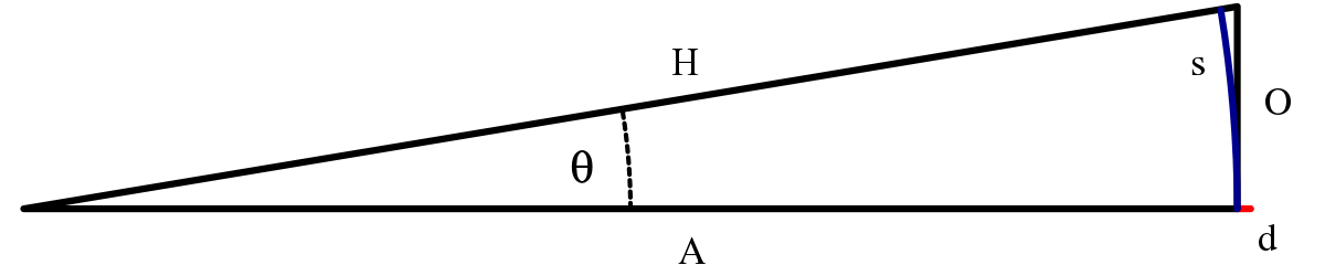 As you probably remember, sine = opposite / hypotenuse = O/H. For small θ, the arc s is very close to O in length, so we can say s ≈ O. The formula for arc length is rθ, where r is the radius of the circle, which is essentially H. So if s ≈ O and s ≈ H θ, then O ≈ H θ, and θ ≈ O / H ≈ sin(θ). By similar logic, we can say that s ≈ A θ, so θ ≈ A / H ≈ tan(θ).
The next method of derivation involves a bit of calculus called L'Hopital's rule. Check out Long Him's article on limits if you haven't encountered the concept before. This rule allows you to find the limits of functions as they approach a point at which they are undefined. Formally stated, if lim(x --> 0) f(x) = 0 and lim(x --> 0) g(x) = 0, then f(x)/g(x) is undefined, but lim(x --> 0) [f(x)/g(x)] = lim(x --> 0) [f'(x)/g'(x)], where f'(x) is the derivative of f(x). In the context of the small angle rule, we are trying to show that lim(x --> 0) [sin(x)/x] = 1, as this would imply that sin(x) = x for small x. sin(x) differentiates to cos(x) and x differentiates to 1, so applying L'Hopital's rule gives us lim(x --> 0) [sin(x)/x] = lim(x --> 0) [cos(x)/1] = lim(x --> 0) [cos(0)] = 1, as required. Similar logic using tan(x) gives lim(x --> 0) [sec^2(x)/1] = lim(x --> 0) [sec^2(0)] = 1. Our final method involves Maclaurin series, which you may have read about in Malhar's article where he uses them to prove Euler's identity. The Maclaurin series for sin(x) is x + (x^3 / 3!) + (x^5 / 5!) + ... and for small values of x, it is valid to truncate the series after the first term, yielding sin(x) ≈ x once again. Similarly, the Maclaurin series for tan(x) is x + (x^3 / 3) + (2/15 x^5) + ... and we can truncate this to give tan(x) ≈ x as required. Hopefully you found this article helpful! Let us know in the comments if you would like to learn about how the small angle rule is applied. Malhar Rajpal  Most of us believe this fascinating finding without even questioning whether it is really true for ALL right angled triangles, and if it is, why it actually works. In this article, I will be showing you my favorite proof of the Pythagorean theorem!  Let’s say we have a square with side length a+b. We can split each side into length a and length b as shown in the diagram above. If we connect each of the splitting points (the dot in between a and b on both sides), we can see 4 right triangles which are similar since they all have sides a and b and have a right angle, as well as an additional quadrilateral area. Because the triangles are similar , we can say the third side of each of these triangles is the same length, which we can call c. This is shown in the diagram below:  To show that the quadrilateral in the centre of the diagram is a square, we need to show that it has equal side lengths (which we have already done, each side has length c), but we also need to show that it has equal angles. Since all four ABC triangles are similar and right angled, we can say that each angle enclosed by sides b and c is called θ and thus the side enclosed by the sides a and c must be equal to 180 - 90 - θ = 90 - θ, since the angles of a triangle must add up to 180 degrees. This is shown in the next diagram:  Since each side on the external square is a straight line, we can say that 90 - θ + θ + x = 180, with x being one angle of the quadrilateral surrounded by the lengths c. By solving this, we can see that x = 90 degrees, a right angle. Since there are four sides and four angles, and since all of them must be x, 90 degrees, the quadrilateral is thus proven to be a square:  So now we can compare areas. We can see the entire area of the external square is (a+b)^2 since each side of the external square is a+b. We can also represent this area as the sum of the areas of the four triangles with side lengths a, b and c and the square with side length c.
The area of the triangles is 4*(1/2)*a*b = 2ab The area of the square is c^2 So we can say (a+b)^2 = c^2 + 2ab Expanding the LHS gives a^2 + 2ab + b^2 = c^2 + 2ab, which cancels to a^2 + b^2 = c^2. This is Pythagoras' theorem! Although the theorem is named the Pythagorean Theorem after the famous Greek philosopher Pythagoras, its actual roots are actually unknown and widely debated. I have shown you one proof of the Pythagorean theorem in this article, but there are actually numerous different proofs, ranging from complex geometric proofs by extremely famed mathematicians to Einstein’s proof by dissection without rearrangement, and proofs using algebra and differentials! The uses for Pythagorean theorem are innumerable and that is why it is so famous! After all, if you are going to use it throughout your secondary education and beyond, you should know why it works! Nitya Nigam Even with COVID-19 lockdowns enforced around the world, there are plenty of virtual opportunities for you to participate in from home. From competitions to communal research projects, there's something out there for every level of aspiring mathematician. In this article, I've compiled a few such opportunities that I've personally found to be engaging.
CrowdMath An open research project aimed at high school and college students, CrowdMath is a collaboration between MIT PRIMES (a high school maths research program run by MIT) and Art of Problem Solving (a great resource that we've recommended in the past). It offers the opportunity to collaborate with peers from around the globe with expert research mentors. Their goal is to create a place for students to experience research mathematics and discover ideas that did not exist before. The topic for 2020 was Metric Dimension, and featured a variety of unanswered questions in graph theory. You can collaborate with other participants via threads on the public message board, so it's really easy to work with each other and ask for help. Definitely something to check out once 2021's topic is announced! International Youth Math Challenge (IYMC) IYMC is an international online maths competitions for secondary school and university students globally (although open to university students, the problems are accessible to most high school maths students). It has three rounds, the first two of which require full written solutions, making it a great way to practice your proof-writing and mathematical communication. You also get an extra commendation if your solutions to the first round are typeset using software like LaTeX, which is wonderful preparation if you intend to study maths (or any mathematical subject, like physics, engineering or computer science) at university, as many of your problem sets will have to be formatted with LaTeX-formatted. Dates for the 2021 competition haven't been released yet, but stay tuned so that you can register when they are! Mathcon Usually attracting 50,000 or so participants annually from schools across the US and worldwide, Mathcon is going virtual this year, offering a 45 minute competition for kids aged 9 to 18. Students who do well qualify for increasingly competitive rounds, eventually reaching the prestigious final. Although this is a paid competition (individual entry is 15USD), winners can earn medals, scholarships and other prizes. The testing window this year is January 19th to March 12th, so make sure to register before the 19th if you're interested! Let us know in the comments if you'd like more recommendations for maths competitions and such! |